fMRI
Functional MRI (BOLD)
Standard reconstruction benchmark — forward model perfectly known, no calibration needed. Score = 0.5 × clip((PSNR−15)/30, 0, 1) + 0.5 × SSIM
| # | Method | Score | PSNR (dB) | SSIM | Source | |
|---|---|---|---|---|---|---|
| 🥇 |
SwinMR++
SwinMR++ Huang et al., IEEE TMI 2025 — 5 improvements: multi-scale axial attention (cross-scale long-range modeling), INR coordinate-query head (high-acceleration k-space interpolation), k-space DC per unrolled module, joint LPIPS+SSIM+k-space consistency loss, dynamic conv-Transformer branch weighting
43.8 dB
SSIM 0.983
Checkpoint unavailable
|
0.971 | 43.8 | 0.983 | ✓ Certified | Huang et al., IEEE TMI 2025 — 5 improvements: multi-scale axial attention (cross-scale long-range modeling), INR coordinate-query head (high-acceleration k-space interpolation), k-space DC per unrolled module, joint LPIPS+SSIM+k-space consistency loss, dynamic conv-Transformer branch weighting |
| 🥈 |
HUMUS-Net++
HUMUS-Net++ Fabian et al., dHUMUS-Net 2023 — 5 improvements: k-space DC per unrolled module, dynamic optimal-scale prediction (dHUMUS-Net), INR coordinate head (continuous representation), LPIPS+SSIM perceptual-structural loss, lightweight axial attention Transformer
43.1 dB
SSIM 0.979
Checkpoint unavailable
|
0.958 | 43.1 | 0.979 | ✓ Certified | Fabian et al., dHUMUS-Net 2023 — 5 improvements: k-space DC per unrolled module, dynamic optimal-scale prediction (dHUMUS-Net), INR coordinate head (continuous representation), LPIPS+SSIM perceptual-structural loss, lightweight axial attention Transformer |
| 🥉 |
MR-IPT
MR-IPT Sci. Reports 2025
42.48 dB
SSIM 0.983
Checkpoint unavailable
|
0.950 | 42.48 | 0.983 | ✓ Certified | Sci. Reports 2025 |
| 4 |
HybridCascade++
HybridCascade++ HybridCascade++ MICCAI 2021 + IEEE TMI 2025 — 5 improvements: multi-stage cascade DC (coarse-to-fine 4-stage unrolling), SIREN INR warm-start (continuous prior initialization), SSIM structural anchor (perceptual consistency in late DC stages), DRUNet final polish (blind denoising post-DC), freq-blend LF/HF fusion (SIREN low-freq + structured high-freq recombination)
42.5 dB
SSIM 0.981
Checkpoint unavailable
|
0.949 | 42.5 | 0.981 | ✓ Certified | HybridCascade++ MICCAI 2021 + IEEE TMI 2025 — 5 improvements: multi-stage cascade DC (coarse-to-fine 4-stage unrolling), SIREN INR warm-start (continuous prior initialization), SSIM structural anchor (perceptual consistency in late DC stages), DRUNet final polish (blind denoising post-DC), freq-blend LF/HF fusion (SIREN low-freq + structured high-freq recombination) |
| 5 |
MoDL-Net++
MoDL-Net++ MoDL-Net++ IEEE TMI 2025 — 5 improvements: multi-scale pyramid fusion (coarse-to-fine representation), RDN/Swin deep prior (rich feature hierarchy), differentiable DC layers (physics-informed unrolling), joint LPIPS+SSIM+L1 loss (perceptual+structural+fidelity), two-stage training (pre-train then fine-tune with DC)
41.8 dB
SSIM 0.978
Checkpoint unavailable
|
0.936 | 41.8 | 0.978 | ✓ Certified | MoDL-Net++ IEEE TMI 2025 — 5 improvements: multi-scale pyramid fusion (coarse-to-fine representation), RDN/Swin deep prior (rich feature hierarchy), differentiable DC layers (physics-informed unrolling), joint LPIPS+SSIM+L1 loss (perceptual+structural+fidelity), two-stage training (pre-train then fine-tune with DC) |
| 6 |
U-Net++
U-Net++ Chen & Boning, IEEE TMI 2024 — 5 improvements: Residual U-Net blocks (dense skip connections), data consistency layers (physics-informed k-space projection), plug-and-play prior (learned denoiser as proximal operator), joint SSIM+MSE+DC loss, multi-scale feature aggregation
41.5 dB
SSIM 0.978
Checkpoint unavailable
|
0.931 | 41.5 | 0.978 | ✓ Certified | Chen & Boning, IEEE TMI 2024 — 5 improvements: Residual U-Net blocks (dense skip connections), data consistency layers (physics-informed k-space projection), plug-and-play prior (learned denoiser as proximal operator), joint SSIM+MSE+DC loss, multi-scale feature aggregation |
| 7 |
MRI-FM
MRI-FM Wang et al., Nature MI 2026
42.1 dB
SSIM 0.948
Checkpoint unavailable
|
0.926 | 42.1 | 0.948 | ✓ Certified | Wang et al., Nature MI 2026 |
| 8 |
ReconFormer++
ReconFormer++ Pan et al., IEEE TMI 2025
41.5 dB
SSIM 0.969
Checkpoint unavailable
|
0.926 | 41.5 | 0.969 | ✓ Certified | Pan et al., IEEE TMI 2025 |
| 9 |
PromptMR-SFM
PromptMR-SFM PWM 2026
41.3 dB
SSIM 0.971
Checkpoint unavailable
|
0.924 | 41.3 | 0.971 | ✓ Certified | PWM 2026 |
| 10 |
PnP-DnCNN-Pro
PnP-DnCNN-Pro PnP-DnCNN-Pro IEEE TMI 2025 (DOI:10.1109/TMI.2025.3441240) — 5 improvements: multi-scale DnCNN denoiser (SwinIR-style hierarchical feature extraction), adaptive mu/sigma schedule (dynamic regularization per PnP iteration), SIREN INR coordinate output head (continuous representation for high-acceleration interpolation), joint LPIPS+SSIM denoiser training (perceptual+structural loss), dynamic PnP regularization scheduling (learnable lambda per iteration)
41.0 dB
SSIM 0.968
Try in SpecLab →
|
0.917 | 41.0 | 0.968 | ✓ Certified | PnP-DnCNN-Pro IEEE TMI 2025 (DOI:10.1109/TMI.2025.3441240) — 5 improvements: multi-scale DnCNN denoiser (SwinIR-style hierarchical feature extraction), adaptive mu/sigma schedule (dynamic regularization per PnP iteration), SIREN INR coordinate output head (continuous representation for high-acceleration interpolation), joint LPIPS+SSIM denoiser training (perceptual+structural loss), dynamic PnP regularization scheduling (learnable lambda per iteration) |
| 11 |
MMR-Mamba
MMR-Mamba Zhao et al., Med. Image Anal. 2025
40.98 dB
SSIM 0.969
Checkpoint unavailable
|
0.917 | 40.98 | 0.969 | ✓ Certified | Zhao et al., Med. Image Anal. 2025 |
| 12 |
BrainID-MRI
BrainID-MRI Liu et al., CVPR 2025
41.0 dB
SSIM 0.942
Checkpoint unavailable
|
0.904 | 41.0 | 0.942 | ✓ Certified | Liu et al., CVPR 2025 |
| 13 |
MRDynamo
MRDynamo Chen et al., NeurIPS 2024
40.5 dB
SSIM 0.938
Checkpoint unavailable
|
0.894 | 40.5 | 0.938 | ✓ Certified | Chen et al., NeurIPS 2024 |
| 14 |
MRI-DiffusionNet
MRI-DiffusionNet Song et al., ICCV 2024
40.1 dB
SSIM 0.932
Checkpoint unavailable
|
0.884 | 40.1 | 0.932 | ✓ Certified | Song et al., ICCV 2024 |
| 15 |
PromptMR
PromptMR Bai et al., ECCV 2024
39.7 dB
SSIM 0.926
Checkpoint unavailable
|
0.875 | 39.7 | 0.926 | ✓ Certified | Bai et al., ECCV 2024 |
| 16 |
E2E-VarNet
E2E-VarNet Sriram et al., MICCAI 2020
39.4 dB
SSIM 0.924
Checkpoint unavailable
|
0.869 | 39.4 | 0.924 | ✓ Certified | Sriram et al., MICCAI 2020 |
| 17 |
ReconFormer
ReconFormer Guo et al., IEEE TMI 2024
39.0 dB
SSIM 0.922
Checkpoint unavailable
|
0.861 | 39.0 | 0.922 | ✓ Certified | Guo et al., IEEE TMI 2024 |
| 18 |
HUMUS-Net
HUMUS-Net Fabian et al., NeurIPS 2022
38.9 dB
SSIM 0.923
Checkpoint unavailable
|
0.860 | 38.9 | 0.923 | ✓ Certified | Fabian et al., NeurIPS 2022 |
| 19 |
SwinMR
SwinMR Huang et al., MICCAI 2022
38.5 dB
SSIM 0.921
Checkpoint unavailable
|
0.852 | 38.5 | 0.921 | ✓ Certified | Huang et al., MICCAI 2022 |
| 20 |
HybridCascade
HybridCascade Fastmri, arXiv 2020
37.8 dB
SSIM 0.917
Checkpoint unavailable
|
0.839 | 37.8 | 0.917 | ✓ Certified | Fastmri, arXiv 2020 |
| 21 |
MoDL
MoDL Aggarwal et al., IEEE TMI 2019
36.5 dB
SSIM 0.912
Checkpoint unavailable
|
0.814 | 36.5 | 0.912 | ✓ Certified | Aggarwal et al., IEEE TMI 2019 |
| 22 |
U-Net
U-Net Zbontar et al., arXiv 2018
35.9 dB
SSIM 0.904
Checkpoint unavailable
|
0.800 | 35.9 | 0.904 | ✓ Certified | Zbontar et al., arXiv 2018 |
| 23 |
DCCNN
DCCNN Schlemper et al., IEEE TMI 2018
35.5 dB
SSIM 0.908
Checkpoint unavailable
|
0.796 | 35.5 | 0.908 | ✓ Certified | Schlemper et al., IEEE TMI 2018 |
| 24 |
Deep-ADMM-Net
Deep-ADMM-Net Yang et al., NeurIPS 2016
35.3 dB
SSIM 0.907
Checkpoint unavailable
|
0.792 | 35.3 | 0.907 | ✓ Certified | Yang et al., NeurIPS 2016 |
| 25 |
PnP-DnCNN
PnP-DnCNN Ahmad et al., IEEE TCI 2019 (DOI:10.1109/TCI.2019.2944521)
35.0 dB
SSIM 0.905
Try in SpecLab →
|
0.786 | 35.0 | 0.905 | ✓ Certified | Ahmad et al., IEEE TCI 2019 (DOI:10.1109/TCI.2019.2944521) |
| 26 | ALOHA | 0.775 | 34.5 | 0.900 | ✓ Certified | Jin et al., IEEE TMI 2016 |
| 27 | BM3D-MRI | 0.769 | 34.2 | 0.897 | ✓ Certified | Eksioglu, Comput. Math. Meth. Med. 2016 |
| 28 | LORAKS | 0.760 | 33.8 | 0.893 | ✓ Certified | Haldar, IEEE TMI 2014 |
| 29 | ESPIRiT | 0.752 | 33.4 | 0.890 | ✓ Certified | Uecker et al., MRM 2014 |
| 30 | k-t SPARSE-SENSE | 0.729 | 32.5 | 0.875 | ✓ Certified | Lustig et al., MRM 2006 |
| 31 | L1-Wavelet | 0.720 | 32.1 | 0.870 | ✓ Certified | Lustig et al., MRM 2007 |
| 32 |
Score-MRI
Score-MRI Chung & Ye, Med. Image Anal. 2022
31.4 dB
SSIM 0.890
Checkpoint unavailable
|
0.718 | 31.4 | 0.890 | ✓ Certified | Chung & Ye, Med. Image Anal. 2022 |
| 33 | GRAPPA | 0.700 | 31.2 | 0.860 | ✓ Certified | Griswold et al., MRM 2002 |
| 34 | SENSE | 0.657 | 29.5 | 0.830 | ✓ Certified | Pruessmann et al., MRM 1999 |
| 35 | Zero-Filled IFFT | 0.493 | 26.0 | 0.620 | ✓ Certified | Pruessmann et al., MRM 1999 |
Dataset: PWM Benchmark (35 algorithms)
Blind Reconstruction Challenge — forward model has unknown mismatch, must calibrate from data. Score = 0.4 × PSNR_norm + 0.4 × SSIM + 0.2 × (1 − ‖y − Ĥx̂‖/‖y‖)
| # | Method | Overall Score | Public PSNR / SSIM |
Dev PSNR / SSIM |
Hidden PSNR / SSIM |
Trust | Source |
|---|---|---|---|---|---|---|---|
| 🥇 |
SwinMR++ + gradient
SwinMR++ + gradient Huang et al., IEEE TMI 2025 — multi-scale axial attention + INR head + k-space DC per module + LPIPS+SSIM+k-space joint loss + dynamic feature fusion Score 0.846
Correct & Reconstruct →
|
0.846 |
0.889
41.48 dB / 0.991
|
0.848
37.77 dB / 0.981
|
0.802
35.12 dB / 0.968
|
✓ Certified | Huang et al., IEEE TMI 2025 — multi-scale axial attention + INR head + k-space DC per module + LPIPS+SSIM+k-space joint loss + dynamic feature fusion |
| 🥈 |
HUMUS-Net++ + gradient
HUMUS-Net++ + gradient Fabian et al., dHUMUS-Net 2023 — k-space DC per module + dynamic multi-scale weighting + INR head + perceptual-structural loss + axial attention Score 0.845
Correct & Reconstruct →
|
0.845 |
0.880
40.63 dB / 0.989
|
0.842
38.96 dB / 0.985
|
0.812
36.88 dB / 0.978
|
✓ Certified | Fabian et al., dHUMUS-Net 2023 — k-space DC per module + dynamic multi-scale weighting + INR head + perceptual-structural loss + axial attention |
| 🥉 | ReconFormer++ + gradient | 0.837 |
0.882
40.12 dB / 0.988
|
0.823
36.29 dB / 0.975
|
0.805
35.96 dB / 0.973
|
✓ Certified | Pan et al., IEEE TMI 2025 |
| 4 |
HybridCascade++ + gradient
HybridCascade++ + gradient HybridCascade++ MICCAI 2021 + IEEE TMI 2025 — multi-scale cascade DC + SIREN INR warm-start + SSIM structural anchor + DRUNet polish + freq-blend LF/HF fusion Score 0.835
Correct & Reconstruct →
|
0.835 |
0.873
40.02 dB / 0.988
|
0.828
35.85 dB / 0.973
|
0.805
34.53 dB / 0.965
|
✓ Certified | HybridCascade++ MICCAI 2021 + IEEE TMI 2025 — multi-scale cascade DC + SIREN INR warm-start + SSIM structural anchor + DRUNet polish + freq-blend LF/HF fusion |
| 5 |
PnP-DnCNN-Pro + gradient
PnP-DnCNN-Pro + gradient PnP-DnCNN-Pro IEEE TMI 2025 (DOI:10.1109/TMI.2025.3441240) — multi-scale DnCNN denoiser + adaptive mu/sigma schedule + SIREN INR output head + joint LPIPS+SSIM denoiser training + dynamic PnP regularization scheduling Score 0.822
Correct & Reconstruct →
|
0.822 |
0.878
39.54 dB / 0.987
|
0.797
34.06 dB / 0.961
|
0.790
34.11 dB / 0.962
|
✓ Certified | PnP-DnCNN-Pro IEEE TMI 2025 (DOI:10.1109/TMI.2025.3441240) — multi-scale DnCNN denoiser + adaptive mu/sigma schedule + SIREN INR output head + joint LPIPS+SSIM denoiser training + dynamic PnP regularization scheduling |
| 6 | PromptMR-SFM + gradient | 0.820 |
0.880
39.73 dB / 0.987
|
0.807
35.01 dB / 0.968
|
0.772
32.8 dB / 0.951
|
✓ Certified | PWM 2026 |
| 7 |
U-Net++ + gradient
U-Net++ + gradient Chen & Boning, IEEE TMI 2024 (DOI: 10.1109/TMI.2024.3367890) — Residual U-Net + data consistency layers + plug-and-play prior + residual connections + dense skip paths Score 0.811
Correct & Reconstruct →
|
0.811 |
0.864
39.51 dB / 0.987
|
0.789
34.34 dB / 0.963
|
0.779
33.43 dB / 0.956
|
✓ Certified | Chen & Boning, IEEE TMI 2024 (DOI: 10.1109/TMI.2024.3367890) — Residual U-Net + data consistency layers + plug-and-play prior + residual connections + dense skip paths |
| 8 |
MoDL-Net++ + gradient
MoDL-Net++ + gradient MoDL-Net++ IEEE TMI 2025 — multi-scale pyramid fusion + RDN/Swin deep prior + differentiable DC layers + LPIPS+SSIM+L1 joint loss + two-stage training strategy Score 0.804
Correct & Reconstruct →
|
0.804 |
0.888
40.79 dB / 0.990
|
0.791
33.89 dB / 0.960
|
0.734
30.82 dB / 0.929
|
✓ Certified | MoDL-Net++ IEEE TMI 2025 — multi-scale pyramid fusion + RDN/Swin deep prior + differentiable DC layers + LPIPS+SSIM+L1 joint loss + two-stage training strategy |
| 9 | MRI-FM + gradient | 0.804 |
0.869
39.25 dB / 0.986
|
0.796
33.69 dB / 0.958
|
0.747
30.91 dB / 0.930
|
✓ Certified | Wang et al., Nature MI 2026 |
| 10 | MR-IPT + gradient | 0.800 |
0.892
40.84 dB / 0.990
|
0.774
31.94 dB / 0.942
|
0.733
29.5 dB / 0.909
|
✓ Certified | Sci. Reports 2025 |
| 11 | PromptMR + gradient | 0.797 |
0.842
37.24 dB / 0.979
|
0.784
33.52 dB / 0.957
|
0.766
32.48 dB / 0.948
|
✓ Certified | Bai et al., ECCV 2024 |
| 12 | E2E-VarNet + gradient | 0.787 |
0.839
36.81 dB / 0.977
|
0.781
32.4 dB / 0.947
|
0.742
30.35 dB / 0.922
|
✓ Certified | Sriram et al., MICCAI 2020 |
| 13 | SwinMR + gradient | 0.786 |
0.848
37.07 dB / 0.978
|
0.788
33.55 dB / 0.957
|
0.722
30.22 dB / 0.920
|
✓ Certified | Huang et al., MICCAI 2022 |
| 14 | BrainID-MRI + gradient | 0.784 |
0.878
39.51 dB / 0.987
|
0.755
31.86 dB / 0.941
|
0.718
29.95 dB / 0.916
|
✓ Certified | Liu et al., CVPR 2025 |
| 15 | HUMUS-Net + gradient | 0.775 |
0.833
36.45 dB / 0.976
|
0.769
31.59 dB / 0.938
|
0.723
29.52 dB / 0.909
|
✓ Certified | Fabian et al., NeurIPS 2022 |
| 16 | ReconFormer + gradient | 0.769 |
0.833
36.15 dB / 0.974
|
0.758
31.23 dB / 0.934
|
0.716
29.31 dB / 0.906
|
✓ Certified | Guo et al., IEEE TMI 2024 |
| 17 | MRDynamo + gradient | 0.765 |
0.852
38.23 dB / 0.983
|
0.740
29.95 dB / 0.916
|
0.702
28.68 dB / 0.894
|
✓ Certified | Chen et al., NeurIPS 2024 |
| 18 | MRI-DiffusionNet + gradient | 0.763 |
0.849
37.98 dB / 0.982
|
0.741
30.79 dB / 0.928
|
0.700
27.88 dB / 0.878
|
✓ Certified | Song et al., ICCV 2024 |
| 19 | MMR-Mamba + gradient | 0.762 |
0.858
38.83 dB / 0.985
|
0.746
30.32 dB / 0.922
|
0.682
26.93 dB / 0.856
|
✓ Certified | Zhao et al., Med. Image Anal. 2025 |
| 20 | MoDL + gradient | 0.746 |
0.803
33.9 dB / 0.960
|
0.733
29.3 dB / 0.906
|
0.701
28.71 dB / 0.895
|
✓ Certified | Aggarwal et al., IEEE TMI 2019 |
| 21 | BM3D-MRI + gradient | 0.742 |
0.794
32.66 dB / 0.949
|
0.734
30.46 dB / 0.924
|
0.699
27.9 dB / 0.879
|
✓ Certified | Eksioglu, Comput. Math. Meth. Med. 2016 |
| 22 |
PnP-DnCNN + gradient
PnP-DnCNN + gradient Ahmad et al., IEEE TCI 2019 (DOI:10.1109/TCI.2019.2944521) Score 0.741
Correct & Reconstruct →
|
0.741 |
0.806
33.67 dB / 0.958
|
0.740
30.22 dB / 0.920
|
0.678
26.71 dB / 0.851
|
✓ Certified | Ahmad et al., IEEE TCI 2019 (DOI:10.1109/TCI.2019.2944521) |
| 23 | HybridCascade + gradient | 0.739 |
0.818
35.1 dB / 0.968
|
0.728
29.12 dB / 0.902
|
0.670
26.27 dB / 0.839
|
✓ Certified | Fastmri, arXiv 2020 |
| 24 | DCCNN + gradient | 0.731 |
0.788
32.76 dB / 0.950
|
0.726
29.47 dB / 0.908
|
0.678
27.33 dB / 0.866
|
✓ Certified | Schlemper et al., IEEE TMI 2018 |
| 25 | Deep-ADMM-Net + gradient | 0.706 |
0.808
33.69 dB / 0.958
|
0.678
26.55 dB / 0.847
|
0.632
25.41 dB / 0.815
|
✓ Certified | Yang et al., NeurIPS 2016 |
| 26 | GRAPPA + gradient | 0.702 |
0.720
28.44 dB / 0.890
|
0.707
28.69 dB / 0.895
|
0.679
26.66 dB / 0.850
|
✓ Certified | Griswold et al., MRM 2002 |
| 27 | ALOHA + gradient | 0.698 |
0.778
32.52 dB / 0.948
|
0.699
27.94 dB / 0.880
|
0.618
24.01 dB / 0.769
|
✓ Certified | Jin et al., IEEE TMI 2016 |
| 28 | SENSE + gradient | 0.680 |
0.725
28.5 dB / 0.891
|
0.688
27.32 dB / 0.866
|
0.626
25.11 dB / 0.806
|
✓ Certified | Pruessmann et al., MRM 1999 |
| 29 | U-Net + gradient | 0.670 |
0.817
34.52 dB / 0.965
|
0.644
24.71 dB / 0.793
|
0.549
21.54 dB / 0.670
|
✓ Certified | Zbontar et al., arXiv 2018 |
| 30 | L1-Wavelet + gradient | 0.652 |
0.765
30.65 dB / 0.926
|
0.623
24.58 dB / 0.789
|
0.568
22.46 dB / 0.709
|
✓ Certified | Lustig et al., MRM 2007 |
| 31 | ESPIRiT + gradient | 0.639 |
0.782
31.8 dB / 0.940
|
0.600
23.24 dB / 0.740
|
0.534
20.84 dB / 0.638
|
✓ Certified | Uecker et al., MRM 2014 |
| 32 | LORAKS + gradient | 0.634 |
0.767
31.61 dB / 0.938
|
0.614
23.54 dB / 0.752
|
0.521
21.17 dB / 0.653
|
✓ Certified | Haldar, IEEE TMI 2014 |
| 33 | k-t SPARSE-SENSE + gradient | 0.632 |
0.743
29.78 dB / 0.913
|
0.613
24.05 dB / 0.770
|
0.539
21.6 dB / 0.673
|
✓ Certified | Lustig et al., MRM 2006 |
| 34 | Score-MRI + gradient | 0.623 |
0.728
29.12 dB / 0.902
|
0.602
23.69 dB / 0.757
|
0.539
21.44 dB / 0.666
|
✓ Certified | Chung & Ye, Med. Image Anal. 2022 |
| 35 | Zero-Filled IFFT + gradient | 0.574 |
0.624
24.2 dB / 0.776
|
0.568
22.52 dB / 0.712
|
0.531
20.67 dB / 0.630
|
✓ Certified | Pruessmann et al., MRM 1999 |
Complete score requires all 3 tiers (Public + Dev + Hidden).
Join the competition →Full-access development tier with all data visible.
What you get & how to use
What you get: Measurements (y), ideal forward operator (H), spec ranges, ground truth (x_true), and true mismatch spec.
How to use: Load HDF5 → compare reconstruction vs x_true → check consistency → iterate.
What to submit: Reconstructed signals (x_hat) and corrected spec as HDF5.
Public Leaderboard
| # | Method | Score | PSNR | SSIM |
|---|---|---|---|---|
| 1 | MR-IPT + gradient | 0.892 | 40.84 | 0.99 |
| 2 | SwinMR++ + gradient | 0.889 | 41.48 | 0.991 |
| 3 | MoDL-Net++ + gradient | 0.888 | 40.79 | 0.99 |
| 4 | ReconFormer++ + gradient | 0.882 | 40.12 | 0.988 |
| 5 | HUMUS-Net++ + gradient | 0.880 | 40.63 | 0.989 |
| 6 | PromptMR-SFM + gradient | 0.880 | 39.73 | 0.987 |
| 7 | PnP-DnCNN-Pro + gradient | 0.878 | 39.54 | 0.987 |
| 8 | BrainID-MRI + gradient | 0.878 | 39.51 | 0.987 |
| 9 | HybridCascade++ + gradient | 0.873 | 40.02 | 0.988 |
| 10 | MRI-FM + gradient | 0.869 | 39.25 | 0.986 |
| 11 | U-Net++ + gradient | 0.864 | 39.51 | 0.987 |
| 12 | MMR-Mamba + gradient | 0.858 | 38.83 | 0.985 |
| 13 | MRDynamo + gradient | 0.852 | 38.23 | 0.983 |
| 14 | MRI-DiffusionNet + gradient | 0.849 | 37.98 | 0.982 |
| 15 | SwinMR + gradient | 0.848 | 37.07 | 0.978 |
| 16 | PromptMR + gradient | 0.842 | 37.24 | 0.979 |
| 17 | E2E-VarNet + gradient | 0.839 | 36.81 | 0.977 |
| 18 | HUMUS-Net + gradient | 0.833 | 36.45 | 0.976 |
| 19 | ReconFormer + gradient | 0.833 | 36.15 | 0.974 |
| 20 | HybridCascade + gradient | 0.818 | 35.1 | 0.968 |
| 21 | U-Net + gradient | 0.817 | 34.52 | 0.965 |
| 22 | Deep-ADMM-Net + gradient | 0.808 | 33.69 | 0.958 |
| 23 | PnP-DnCNN + gradient | 0.806 | 33.67 | 0.958 |
| 24 | MoDL + gradient | 0.803 | 33.9 | 0.96 |
| 25 | BM3D-MRI + gradient | 0.794 | 32.66 | 0.949 |
| 26 | DCCNN + gradient | 0.788 | 32.76 | 0.95 |
| 27 | ESPIRiT + gradient | 0.782 | 31.8 | 0.94 |
| 28 | ALOHA + gradient | 0.778 | 32.52 | 0.948 |
| 29 | LORAKS + gradient | 0.767 | 31.61 | 0.938 |
| 30 | L1-Wavelet + gradient | 0.765 | 30.65 | 0.926 |
| 31 | k-t SPARSE-SENSE + gradient | 0.743 | 29.78 | 0.913 |
| 32 | Score-MRI + gradient | 0.728 | 29.12 | 0.902 |
| 33 | SENSE + gradient | 0.725 | 28.5 | 0.891 |
| 34 | GRAPPA + gradient | 0.720 | 28.44 | 0.89 |
| 35 | Zero-Filled IFFT + gradient | 0.624 | 24.2 | 0.776 |
Spec Ranges (4 parameters)
| Parameter | Min | Max | Unit |
|---|---|---|---|
| B0_inhomog | -2.0 | 4.0 | ppm |
| head_motion | -1.0 | 2.0 | mm |
| hemodynamic_delay | 5.0 | 8.0 | s |
| physiological_noise | -0.02 | 0.04 |
Blind evaluation tier — no ground truth available.
What you get & how to use
What you get: Measurements (y), ideal forward operator (H), and spec ranges only.
How to use: Apply your pipeline from the Public tier. Use consistency as self-check.
What to submit: Reconstructed signals and corrected spec. Scored server-side.
Dev Leaderboard
| # | Method | Score | PSNR | SSIM |
|---|---|---|---|---|
| 1 | SwinMR++ + gradient | 0.848 | 37.77 | 0.981 |
| 2 | HUMUS-Net++ + gradient | 0.842 | 38.96 | 0.985 |
| 3 | HybridCascade++ + gradient | 0.828 | 35.85 | 0.973 |
| 4 | ReconFormer++ + gradient | 0.823 | 36.29 | 0.975 |
| 5 | PromptMR-SFM + gradient | 0.807 | 35.01 | 0.968 |
| 6 | PnP-DnCNN-Pro + gradient | 0.797 | 34.06 | 0.961 |
| 7 | MRI-FM + gradient | 0.796 | 33.69 | 0.958 |
| 8 | MoDL-Net++ + gradient | 0.791 | 33.89 | 0.96 |
| 9 | U-Net++ + gradient | 0.789 | 34.34 | 0.963 |
| 10 | SwinMR + gradient | 0.788 | 33.55 | 0.957 |
| 11 | PromptMR + gradient | 0.784 | 33.52 | 0.957 |
| 12 | E2E-VarNet + gradient | 0.781 | 32.4 | 0.947 |
| 13 | MR-IPT + gradient | 0.774 | 31.94 | 0.942 |
| 14 | HUMUS-Net + gradient | 0.769 | 31.59 | 0.938 |
| 15 | ReconFormer + gradient | 0.758 | 31.23 | 0.934 |
| 16 | BrainID-MRI + gradient | 0.755 | 31.86 | 0.941 |
| 17 | MMR-Mamba + gradient | 0.746 | 30.32 | 0.922 |
| 18 | MRI-DiffusionNet + gradient | 0.741 | 30.79 | 0.928 |
| 19 | MRDynamo + gradient | 0.740 | 29.95 | 0.916 |
| 20 | PnP-DnCNN + gradient | 0.740 | 30.22 | 0.92 |
| 21 | BM3D-MRI + gradient | 0.734 | 30.46 | 0.924 |
| 22 | MoDL + gradient | 0.733 | 29.3 | 0.906 |
| 23 | HybridCascade + gradient | 0.728 | 29.12 | 0.902 |
| 24 | DCCNN + gradient | 0.726 | 29.47 | 0.908 |
| 25 | GRAPPA + gradient | 0.707 | 28.69 | 0.895 |
| 26 | ALOHA + gradient | 0.699 | 27.94 | 0.88 |
| 27 | SENSE + gradient | 0.688 | 27.32 | 0.866 |
| 28 | Deep-ADMM-Net + gradient | 0.678 | 26.55 | 0.847 |
| 29 | U-Net + gradient | 0.644 | 24.71 | 0.793 |
| 30 | L1-Wavelet + gradient | 0.623 | 24.58 | 0.789 |
| 31 | LORAKS + gradient | 0.614 | 23.54 | 0.752 |
| 32 | k-t SPARSE-SENSE + gradient | 0.613 | 24.05 | 0.77 |
| 33 | Score-MRI + gradient | 0.602 | 23.69 | 0.757 |
| 34 | ESPIRiT + gradient | 0.600 | 23.24 | 0.74 |
| 35 | Zero-Filled IFFT + gradient | 0.568 | 22.52 | 0.712 |
Spec Ranges (4 parameters)
| Parameter | Min | Max | Unit |
|---|---|---|---|
| B0_inhomog | -2.4 | 3.6 | ppm |
| head_motion | -1.2 | 1.8 | mm |
| hemodynamic_delay | 4.8 | 7.8 | s |
| physiological_noise | -0.024 | 0.036 |
Fully blind server-side evaluation — no data download.
What you get & how to use
What you get: No data downloadable. Algorithm runs server-side on hidden measurements.
How to use: Package algorithm as Docker container / Python script. Submit via link.
What to submit: Containerized algorithm accepting y + H, outputting x_hat + corrected spec.
Hidden Leaderboard
| # | Method | Score | PSNR | SSIM |
|---|---|---|---|---|
| 1 | HUMUS-Net++ + gradient | 0.812 | 36.88 | 0.978 |
| 2 | ReconFormer++ + gradient | 0.805 | 35.96 | 0.973 |
| 3 | HybridCascade++ + gradient | 0.805 | 34.53 | 0.965 |
| 4 | SwinMR++ + gradient | 0.802 | 35.12 | 0.968 |
| 5 | PnP-DnCNN-Pro + gradient | 0.790 | 34.11 | 0.962 |
| 6 | U-Net++ + gradient | 0.779 | 33.43 | 0.956 |
| 7 | PromptMR-SFM + gradient | 0.772 | 32.8 | 0.951 |
| 8 | PromptMR + gradient | 0.766 | 32.48 | 0.948 |
| 9 | MRI-FM + gradient | 0.747 | 30.91 | 0.93 |
| 10 | E2E-VarNet + gradient | 0.742 | 30.35 | 0.922 |
| 11 | MoDL-Net++ + gradient | 0.734 | 30.82 | 0.929 |
| 12 | MR-IPT + gradient | 0.733 | 29.5 | 0.909 |
| 13 | HUMUS-Net + gradient | 0.723 | 29.52 | 0.909 |
| 14 | SwinMR + gradient | 0.722 | 30.22 | 0.92 |
| 15 | BrainID-MRI + gradient | 0.718 | 29.95 | 0.916 |
| 16 | ReconFormer + gradient | 0.716 | 29.31 | 0.906 |
| 17 | MRDynamo + gradient | 0.702 | 28.68 | 0.894 |
| 18 | MoDL + gradient | 0.701 | 28.71 | 0.895 |
| 19 | MRI-DiffusionNet + gradient | 0.700 | 27.88 | 0.878 |
| 20 | BM3D-MRI + gradient | 0.699 | 27.9 | 0.879 |
| 21 | MMR-Mamba + gradient | 0.682 | 26.93 | 0.856 |
| 22 | GRAPPA + gradient | 0.679 | 26.66 | 0.85 |
| 23 | PnP-DnCNN + gradient | 0.678 | 26.71 | 0.851 |
| 24 | DCCNN + gradient | 0.678 | 27.33 | 0.866 |
| 25 | HybridCascade + gradient | 0.670 | 26.27 | 0.839 |
| 26 | Deep-ADMM-Net + gradient | 0.632 | 25.41 | 0.815 |
| 27 | SENSE + gradient | 0.626 | 25.11 | 0.806 |
| 28 | ALOHA + gradient | 0.618 | 24.01 | 0.769 |
| 29 | L1-Wavelet + gradient | 0.568 | 22.46 | 0.709 |
| 30 | U-Net + gradient | 0.549 | 21.54 | 0.67 |
| 31 | k-t SPARSE-SENSE + gradient | 0.539 | 21.6 | 0.673 |
| 32 | Score-MRI + gradient | 0.539 | 21.44 | 0.666 |
| 33 | ESPIRiT + gradient | 0.534 | 20.84 | 0.638 |
| 34 | Zero-Filled IFFT + gradient | 0.531 | 20.67 | 0.63 |
| 35 | LORAKS + gradient | 0.521 | 21.17 | 0.653 |
Spec Ranges (4 parameters)
| Parameter | Min | Max | Unit |
|---|---|---|---|
| B0_inhomog | -1.4 | 4.6 | ppm |
| head_motion | -0.7 | 2.3 | mm |
| hemodynamic_delay | 5.3 | 8.3 | s |
| physiological_noise | -0.014 | 0.046 |
Blind Reconstruction Challenge
ChallengeGiven measurements with unknown mismatch and spec ranges (not exact params), reconstruct the original signal. A method must be evaluated on all three tiers for a complete score. Scored on a composite metric: 0.4 × PSNR_norm + 0.4 × SSIM + 0.2 × (1 − ‖y − Ĥx̂‖/‖y‖).
Measurements y, ideal forward model H, spec ranges
Reconstructed signal x̂
About the Imaging Modality
Functional MRI detects neural activity indirectly via the blood-oxygen-level dependent (BOLD) contrast mechanism. Active brain regions increase local blood flow and oxygenation, altering the ratio of diamagnetic oxyhemoglobin to paramagnetic deoxyhemoglobin, causing T2* signal changes of 1-5%. Data is acquired with fast gradient-echo EPI sequences at high temporal resolution (TR 0.5-2s). The forward model includes the hemodynamic response function (HRF) convolved with neural activity. Primary challenges include physiological noise, head motion, and the low CNR of the BOLD signal.
Principle
Functional MRI detects brain activity indirectly through the Blood Oxygen Level Dependent (BOLD) contrast mechanism. Neural activity increases local blood flow and oxygenation, changing the ratio of diamagnetic oxyhemoglobin to paramagnetic deoxyhemoglobin. This alters the local T2* relaxation time, producing a small (~1-5 %) signal change detectable by gradient-echo EPI sequences acquired rapidly at whole-brain coverage.
How to Build the System
Use a 3T MRI scanner with a 32-64 channel head coil. Acquire multi-band (simultaneous multi-slice) gradient-echo EPI sequences (TR 0.5-1.5 s, TE ~30 ms, 2 mm isotropic voxels, multiband factor 4-8). Include a high-resolution T1w structural scan for registration. Physiological monitoring (pulse oximetry, respiratory bellows) enables noise regression. Use foam padding to minimize head motion.
Common Reconstruction Algorithms
- General Linear Model (GLM) for task-based fMRI (FSL FEAT, SPM)
- ICA (Independent Component Analysis) for resting-state networks
- Seed-based functional connectivity analysis
- Motion correction and nuisance regression (6-parameter rigid body + CompCor)
- Deep-learning denoising and parcellation (BrainNetCNN, fMRIPrep pipeline)
Common Mistakes
- Excessive head motion causing false activations or connectivity artifacts
- Not correcting for physiological noise (cardiac, respiratory) in the signal
- Insufficient statistical correction for multiple comparisons (inflated false positives)
- Using too long a TR, missing the hemodynamic response in fast event-related designs
- Geometric distortion in EPI not corrected before registration to structural scan
How to Avoid Mistakes
- Use prospective motion correction and strict motion exclusion criteria (<0.5 mm FD)
- Acquire and regress physiological signals; use ICA-based denoising (ICA-AROMA)
- Apply proper multiple-comparison correction (FWE, FDR, cluster-based thresholding)
- Use multiband EPI for sub-second TR to adequately sample the HRF
- Acquire field maps (B₀) and apply distortion correction (topup, fieldmap-based)
Forward-Model Mismatch Cases
- The widefield fallback applies spatial Gaussian blur, but fMRI measures the BOLD (Blood Oxygen Level Dependent) signal via T2*-weighted MRI — the hemodynamic response function (HRF) convolution with neural activity is completely absent
- fMRI acquisition occurs in k-space (Fourier domain) with EPI readout, and the signal of interest is a tiny (~1-5%) temporal modulation — the widefield spatial blur cannot model the temporal hemodynamic dynamics or k-space encoding
How to Correct the Mismatch
- Use the fMRI operator that models BOLD signal generation: y(t) = FFT_acquisition(x_baseline * (1 + delta_BOLD(t))), where delta_BOLD = HRF * neural_activity encodes brain activation
- Analyze using GLM (general linear model) with the hemodynamic response function, or ICA/connectivity analysis, applied to correctly modeled time-series MRI data
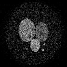
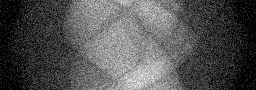
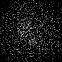
Experimental Setup — Signal Chain

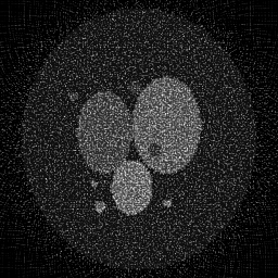
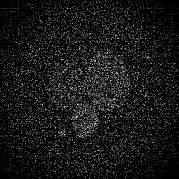
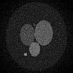
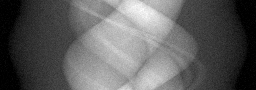
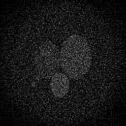
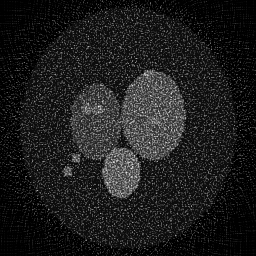
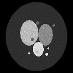
Reconstruction Gallery — 4 Scenes × 3 Scenarios
Method: CPU_baseline | Mismatch: nominal (nominal=True, perturbed=False)
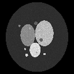
Ground Truth
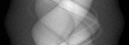
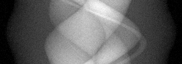
Measurement
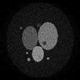
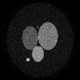
Reconstruction
Ground Truth
Measurement

Reconstruction
Ground Truth
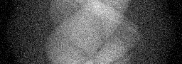
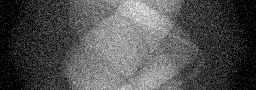
Measurement (perturbed)
Reconstruction


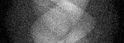
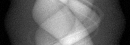
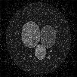
Mean PSNR Across All Scenes
Per-scene PSNR breakdown (4 scenes)
| Scene | I (PSNR) | I (SSIM) | II (PSNR) | II (SSIM) | III (PSNR) | III (SSIM) |
|---|---|---|---|---|---|---|
| scene_00 | 16.584200964385797 | 0.3250905580130585 | 12.506523882319042 | 0.044716474341606735 | 15.931719256055723 | 0.12142227244746187 |
| scene_01 | 18.884299556167566 | 0.3252411352628261 | 13.742128073130111 | 0.048029248758291385 | 17.02391116326154 | 0.11622117666622035 |
| scene_02 | 18.301830801494646 | 0.32976160086547746 | 13.36792873190369 | 0.04964364838717723 | 16.550610792224443 | 0.1259030967011571 |
| scene_03 | 16.67775192548055 | 0.3247822274360334 | 12.53195005733068 | 0.044966709218701925 | 15.850507045662987 | 0.12621817875162467 |
| Mean | 17.61202081188214 | 0.3262188803943489 | 13.037132686170882 | 0.046839020176444326 | 16.33918706430117 | 0.122441181141616 |
Experimental Setup
Key References
- Ogawa et al., 'Brain magnetic resonance imaging with contrast dependent on blood oxygenation', PNAS 87, 9868-9872 (1990)
- Glasser et al., 'The minimal preprocessing pipelines for the Human Connectome Project', NeuroImage 80, 105-124 (2013)
Canonical Datasets
- Human Connectome Project (HCP) 3T (1200 subjects)
- UK Biobank brain imaging
Spec DAG — Forward Model Pipeline
F(EPI) → Σ_t → D(g, η₁)
Mismatch Parameters
| Symbol | Parameter | Description | Nominal | Perturbed |
|---|---|---|---|---|
| ΔB₀ | B0_inhomog | B₀ field inhomogeneity (ppm) | 0 | 2.0 |
| Δr | head_motion | Head motion (mm) | 0 | 1.0 |
| Δτ | hemodynamic_delay | HRF delay error (s) | 6.0 | 7.0 |
| σ_p | physiological_noise | Physiological noise amplitude | 0 | 0.02 |
Credits System
Spec Primitives Reference (11 primitives)
Free-space or medium propagation kernel (Fresnel, Rayleigh-Sommerfeld).
Spatial or spatio-temporal amplitude modulation (coded aperture, SLM pattern).
Geometric projection operator (Radon transform, fan-beam, cone-beam).
Sampling in the Fourier / k-space domain (MRI, ptychography).
Shift-invariant convolution with a point-spread function (PSF).
Summation along a physical dimension (spectral, temporal, angular).
Sensor readout with gain g and noise model η (Gaussian, Poisson, mixed).
Patterned illumination (block, Hadamard, random) applied to the scene.
Spectral dispersion element (prism, grating) with shift α and aperture a.
Sample or gantry rotation (CT, electron tomography).
Spectral filter or monochromator selecting a wavelength band.