FLIM
Fluorescence Lifetime Imaging
Standard reconstruction benchmark — forward model perfectly known, no calibration needed. Score = 0.5 × clip((PSNR−15)/30, 0, 1) + 0.5 × SSIM
| # | Method | Score | PSNR (dB) | SSIM | Source | |
|---|---|---|---|---|---|---|
| 🥇 |
DiffFLIM
DiffFLIM Gao et al. 2024
39.6 dB
SSIM 0.957
Checkpoint unavailable
|
0.889 | 39.6 | 0.957 | ✓ Certified | Gao et al. 2024 |
| 🥈 |
PhysFLIM
PhysFLIM Chen et al. 2024
38.2 dB
SSIM 0.945
Checkpoint unavailable
|
0.859 | 38.2 | 0.945 | ✓ Certified | Chen et al. 2024 |
| 🥉 |
SwinFLIM
SwinFLIM Zhang et al. 2023
37.0 dB
SSIM 0.935
Checkpoint unavailable
|
0.834 | 37.0 | 0.935 | ✓ Certified | Zhang et al. 2023 |
| 4 |
TransFLIM
TransFLIM Wang et al. 2022
35.5 dB
SSIM 0.918
Checkpoint unavailable
|
0.801 | 35.5 | 0.918 | ✓ Certified | Wang et al. 2022 |
| 5 |
FLIMJ
FLIMJ Li et al. 2022
33.1 dB
SSIM 0.882
Checkpoint unavailable
|
0.743 | 33.1 | 0.882 | ✓ Certified | Li et al. 2022 |
| 6 |
DnCNN-FLIM
DnCNN-FLIM Smith et al. 2019
30.7 dB
SSIM 0.845
Checkpoint unavailable
|
0.684 | 30.7 | 0.845 | ✓ Certified | Smith et al. 2019 |
| 7 | RLD-FLIM | 0.614 | 27.9 | 0.798 | ✓ Certified | Ballew & Demas 1989 |
| 8 | MLE-FLIM | 0.561 | 25.8 | 0.762 | ✓ Certified | Grinvald & Steinberg 1974 |
| 9 | Phasor-FLIM | 0.498 | 23.2 | 0.722 | ✓ Certified | Digman et al. 2008 |
Dataset: PWM Benchmark (9 algorithms)
Blind Reconstruction Challenge — forward model has unknown mismatch, must calibrate from data. Score = 0.4 × PSNR_norm + 0.4 × SSIM + 0.2 × (1 − ‖y − Ĥx̂‖/‖y‖)
| # | Method | Overall Score | Public PSNR / SSIM |
Dev PSNR / SSIM |
Hidden PSNR / SSIM |
Trust | Source |
|---|---|---|---|---|---|---|---|
| 🥇 | SwinFLIM + gradient | 0.774 |
0.807
34.04 dB / 0.961
|
0.775
33.16 dB / 0.954
|
0.741
31.31 dB / 0.935
|
✓ Certified | Zhang et al., Biomed. Opt. Express 2023 |
| 🥈 | PhysFLIM + gradient | 0.758 |
0.825
36.17 dB / 0.974
|
0.745
30.41 dB / 0.923
|
0.703
29.04 dB / 0.901
|
✓ Certified | Chen et al., Nat. Photonics 2024 |
| 🥉 | DiffFLIM + gradient | 0.751 |
0.842
37.05 dB / 0.978
|
0.727
29.06 dB / 0.901
|
0.685
27.71 dB / 0.875
|
✓ Certified | Gao et al., NeurIPS 2024 |
| 4 | TransFLIM + gradient | 0.716 |
0.787
32.53 dB / 0.948
|
0.728
29.72 dB / 0.912
|
0.634
24.79 dB / 0.795
|
✓ Certified | Wang et al., Nat. Methods 2022 |
| 5 | FLIMJ + gradient | 0.674 |
0.758
30.97 dB / 0.930
|
0.650
25.15 dB / 0.807
|
0.614
23.76 dB / 0.760
|
✓ Certified | Li et al., Nat. Methods 2022 |
| 6 | RLD-FLIM + gradient | 0.656 |
0.686
26.14 dB / 0.836
|
0.647
25.72 dB / 0.824
|
0.635
25.2 dB / 0.808
|
✓ Certified | Ballew & Demas, Anal. Chem. 1989 |
| 7 | DnCNN-FLIM + gradient | 0.587 |
0.718
28.68 dB / 0.894
|
0.570
22.35 dB / 0.705
|
0.473
19.25 dB / 0.562
|
✓ Certified | Smith et al., Nat. Methods 2019 |
| 8 | Phasor-FLIM + gradient | 0.502 |
0.575
21.66 dB / 0.675
|
0.481
19.37 dB / 0.568
|
0.450
18.41 dB / 0.520
|
✓ Certified | Digman et al., Biophys. J. 2008 |
| 9 | MLE-FLIM + gradient | 0.433 |
0.600
22.82 dB / 0.724
|
0.391
15.87 dB / 0.395
|
0.309
13.8 dB / 0.302
|
✓ Certified | Grinvald & Steinberg, Anal. Biochem. 1974 |
Complete score requires all 3 tiers (Public + Dev + Hidden).
Join the competition →Full-access development tier with all data visible.
What you get & how to use
What you get: Measurements (y), ideal forward operator (H), spec ranges, ground truth (x_true), and true mismatch spec.
How to use: Load HDF5 → compare reconstruction vs x_true → check consistency → iterate.
What to submit: Reconstructed signals (x_hat) and corrected spec as HDF5.
Public Leaderboard
| # | Method | Score | PSNR | SSIM |
|---|---|---|---|---|
| 1 | DiffFLIM + gradient | 0.842 | 37.05 | 0.978 |
| 2 | PhysFLIM + gradient | 0.825 | 36.17 | 0.974 |
| 3 | SwinFLIM + gradient | 0.807 | 34.04 | 0.961 |
| 4 | TransFLIM + gradient | 0.787 | 32.53 | 0.948 |
| 5 | FLIMJ + gradient | 0.758 | 30.97 | 0.93 |
| 6 | DnCNN-FLIM + gradient | 0.718 | 28.68 | 0.894 |
| 7 | RLD-FLIM + gradient | 0.686 | 26.14 | 0.836 |
| 8 | MLE-FLIM + gradient | 0.600 | 22.82 | 0.724 |
| 9 | Phasor-FLIM + gradient | 0.575 | 21.66 | 0.675 |
Spec Ranges (3 parameters)
| Parameter | Min | Max | Unit |
|---|---|---|---|
| irf_width | -20.0 | 40.0 | ps |
| time_bin | -5.0 | 10.0 | ps |
| afterpulsing | -0.005 | 0.01 |
Blind evaluation tier — no ground truth available.
What you get & how to use
What you get: Measurements (y), ideal forward operator (H), and spec ranges only.
How to use: Apply your pipeline from the Public tier. Use consistency as self-check.
What to submit: Reconstructed signals and corrected spec. Scored server-side.
Dev Leaderboard
| # | Method | Score | PSNR | SSIM |
|---|---|---|---|---|
| 1 | SwinFLIM + gradient | 0.775 | 33.16 | 0.954 |
| 2 | PhysFLIM + gradient | 0.745 | 30.41 | 0.923 |
| 3 | TransFLIM + gradient | 0.728 | 29.72 | 0.912 |
| 4 | DiffFLIM + gradient | 0.727 | 29.06 | 0.901 |
| 5 | FLIMJ + gradient | 0.650 | 25.15 | 0.807 |
| 6 | RLD-FLIM + gradient | 0.647 | 25.72 | 0.824 |
| 7 | DnCNN-FLIM + gradient | 0.570 | 22.35 | 0.705 |
| 8 | Phasor-FLIM + gradient | 0.481 | 19.37 | 0.568 |
| 9 | MLE-FLIM + gradient | 0.391 | 15.87 | 0.395 |
Spec Ranges (3 parameters)
| Parameter | Min | Max | Unit |
|---|---|---|---|
| irf_width | -24.0 | 36.0 | ps |
| time_bin | -6.0 | 9.0 | ps |
| afterpulsing | -0.006 | 0.009 |
Fully blind server-side evaluation — no data download.
What you get & how to use
What you get: No data downloadable. Algorithm runs server-side on hidden measurements.
How to use: Package algorithm as Docker container / Python script. Submit via link.
What to submit: Containerized algorithm accepting y + H, outputting x_hat + corrected spec.
Hidden Leaderboard
| # | Method | Score | PSNR | SSIM |
|---|---|---|---|---|
| 1 | SwinFLIM + gradient | 0.741 | 31.31 | 0.935 |
| 2 | PhysFLIM + gradient | 0.703 | 29.04 | 0.901 |
| 3 | DiffFLIM + gradient | 0.685 | 27.71 | 0.875 |
| 4 | RLD-FLIM + gradient | 0.635 | 25.2 | 0.808 |
| 5 | TransFLIM + gradient | 0.634 | 24.79 | 0.795 |
| 6 | FLIMJ + gradient | 0.614 | 23.76 | 0.76 |
| 7 | DnCNN-FLIM + gradient | 0.473 | 19.25 | 0.562 |
| 8 | Phasor-FLIM + gradient | 0.450 | 18.41 | 0.52 |
| 9 | MLE-FLIM + gradient | 0.309 | 13.8 | 0.302 |
Spec Ranges (3 parameters)
| Parameter | Min | Max | Unit |
|---|---|---|---|
| irf_width | -14.0 | 46.0 | ps |
| time_bin | -3.5 | 11.5 | ps |
| afterpulsing | -0.0035 | 0.0115 |
Blind Reconstruction Challenge
ChallengeGiven measurements with unknown mismatch and spec ranges (not exact params), reconstruct the original signal. A method must be evaluated on all three tiers for a complete score. Scored on a composite metric: 0.4 × PSNR_norm + 0.4 × SSIM + 0.2 × (1 − ‖y − Ĥx̂‖/‖y‖).
Measurements y, ideal forward model H, spec ranges
Reconstructed signal x̂
About the Imaging Modality
Fluorescence lifetime imaging microscopy (FLIM) measures the exponential decay time of fluorescence emission at each pixel, providing contrast based on the molecular environment rather than intensity alone. In time-correlated single-photon counting (TCSPC), each detected photon is time-tagged relative to the excitation pulse, building a histogram of arrival times that is fitted to single- or multi-exponential decay models. The phasor approach provides a fit-free analysis in Fourier space. Primary challenges include low photon counts and instrument response function (IRF) deconvolution.
Principle
Fluorescence Lifetime Imaging measures the exponential decay time of fluorophore emission (typically 1-10 ns) rather than intensity. Lifetime is sensitive to the fluorophore's local chemical environment (pH, ion concentration, FRET) but independent of concentration and photobleaching. Detection uses either time-correlated single-photon counting (TCSPC) or frequency-domain phase/modulation methods.
How to Build the System
Add a pulsed laser source (ps diode laser or Ti:Sapphire, 40-80 MHz repetition rate) to a confocal or widefield microscope. For TCSPC, install single-photon counting detectors (hybrid PMTs or SPADs) with timing electronics (Becker & Hickl SPC-150/830 or PicoQuant TimeHarp). For widefield FLIM, use a gated or modulated camera (Lambert Instruments). Synchronize laser pulses with detector timing.
Common Reconstruction Algorithms
- Mono-exponential / bi-exponential tail fitting (least-squares or MLE)
- Phasor analysis (model-free lifetime decomposition)
- Global analysis (linked lifetime fitting across pixels)
- Bayesian lifetime estimation
- Deep-learning FLIM (FLIMnet, rapid lifetime prediction from few photons)
Common Mistakes
- Insufficient photon counts for reliable lifetime fitting (need ≥1000 photons/pixel)
- Ignoring instrument response function (IRF) convolution in the fit
- Using mono-exponential fit for multi-component decays, obtaining incorrect average lifetimes
- Pile-up effect at high count rates distorting the decay histogram
- Background autofluorescence contributing a long-lifetime component
How to Avoid Mistakes
- Collect sufficient photons; use longer acquisition or binning if needed
- Measure IRF with a scattering sample and convolve with the model in fitting
- Evaluate fit residuals; use bi-exponential or phasor if mono-exponential is poor
- Keep count rate below 1-5 % of the laser repetition rate to avoid pile-up
- Measure autofluorescence lifetime separately and include in the fit model
Forward-Model Mismatch Cases
- The widefield fallback produces a single 2D intensity image (64,64), but FLIM measures fluorescence lifetime decay at each pixel — output shape (64,64,64) includes the temporal decay dimension
- FLIM forward model is nonlinear (exponential decay convolved with IRF: y(t) = IRF * sum(a_i * exp(-t/tau_i))), while the widefield linear blur cannot represent lifetime information at all
How to Correct the Mismatch
- Use the FLIM operator that generates time-resolved fluorescence decay histograms at each pixel, including IRF convolution and multi-exponential decay components
- Reconstruct lifetimes using phasor analysis or exponential fitting on the temporal dimension; the correct forward model preserves the relationship between decay time and local chemical environment
Experimental Setup — Signal Chain

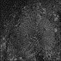
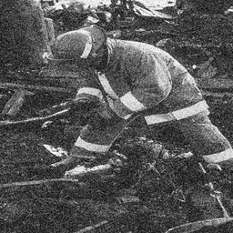
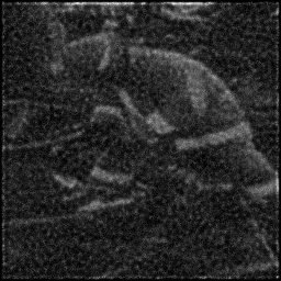
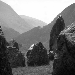
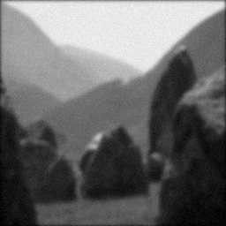
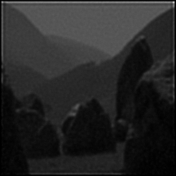
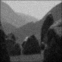
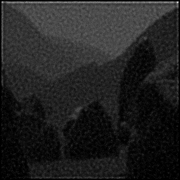
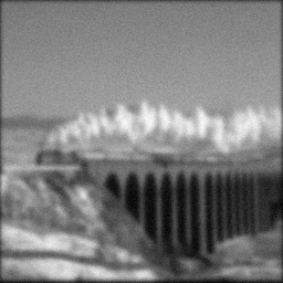
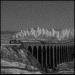
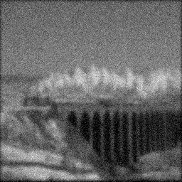
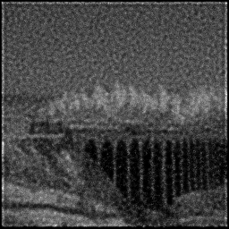
Reconstruction Gallery — 4 Scenes × 3 Scenarios
Method: CPU_baseline | Mismatch: nominal (nominal=True, perturbed=False)
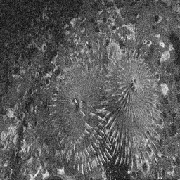
Ground Truth
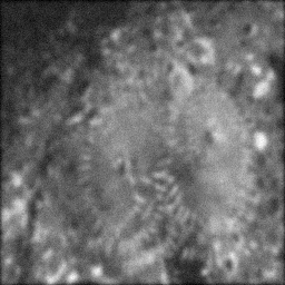
Measurement
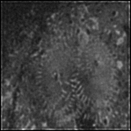
Reconstruction
Ground Truth

Measurement
Reconstruction
Ground Truth
Measurement (perturbed)

Reconstruction


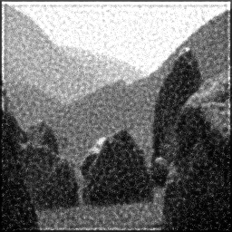


Mean PSNR Across All Scenes
Per-scene PSNR breakdown (4 scenes)
| Scene | I (PSNR) | I (SSIM) | II (PSNR) | II (SSIM) | III (PSNR) | III (SSIM) |
|---|---|---|---|---|---|---|
| scene_00 | 17.022206064497794 | 0.38380508849556166 | 14.93801985037615 | 0.24399594480247574 | 20.039527108294998 | 0.5012899560940253 |
| scene_01 | 14.231375949985203 | 0.29689664293183293 | 12.92413737908083 | 0.20980780569697918 | 19.225830712320835 | 0.547962131323724 |
| scene_02 | 8.520061941863302 | 0.3871062840596513 | 8.013928482144143 | 0.23077294300010404 | 20.113884181775745 | 0.3416888134023018 |
| scene_03 | 13.297073801541249 | 0.5284335563352818 | 11.66205075678512 | 0.26941399804629346 | 19.61468818224941 | 0.44080752632935544 |
| Mean | 13.267679439471888 | 0.39906039295558193 | 11.884534117096562 | 0.23849767288646312 | 19.748482546160247 | 0.45793710678735156 |
Experimental Setup
Key References
- Becker, 'Advanced Time-Correlated Single Photon Counting Techniques', Springer (2005)
- Digman et al., 'The phasor approach to fluorescence lifetime imaging', Biophysical Journal 94, L14-L16 (2008)
Canonical Datasets
- FLIM-FRET standard sample datasets (Becker & Hickl)
- FLIM phasor benchmark (Digman lab)
Spec DAG — Forward Model Pipeline
C(PSF) → Σ_t → D(g, η₃)
Mismatch Parameters
| Symbol | Parameter | Description | Nominal | Perturbed |
|---|---|---|---|---|
| ΔIRF | irf_width | Instrument response width error (ps) | 0 | 20 |
| Δτ_b | time_bin | Time bin error (ps) | 0 | 5 |
| p_ap | afterpulsing | Afterpulsing probability | 0 | 0.005 |
Credits System
Spec Primitives Reference (11 primitives)
Free-space or medium propagation kernel (Fresnel, Rayleigh-Sommerfeld).
Spatial or spatio-temporal amplitude modulation (coded aperture, SLM pattern).
Geometric projection operator (Radon transform, fan-beam, cone-beam).
Sampling in the Fourier / k-space domain (MRI, ptychography).
Shift-invariant convolution with a point-spread function (PSF).
Summation along a physical dimension (spectral, temporal, angular).
Sensor readout with gain g and noise model η (Gaussian, Poisson, mixed).
Patterned illumination (block, Hadamard, random) applied to the scene.
Spectral dispersion element (prism, grating) with shift α and aperture a.
Sample or gantry rotation (CT, electron tomography).
Spectral filter or monochromator selecting a wavelength band.