Endoscopy
Fiber Bundle Endoscopy
Standard reconstruction benchmark — forward model perfectly known, no calibration needed. Score = 0.5 × clip((PSNR−15)/30, 0, 1) + 0.5 × SSIM
| # | Method | Score | PSNR (dB) | SSIM | Source | |
|---|---|---|---|---|---|---|
| 🥇 |
DiffEndo
DiffEndo Gao et al. 2024
39.7 dB
SSIM 0.957
Checkpoint unavailable
|
0.890 | 39.7 | 0.957 | ✓ Certified | Gao et al. 2024 |
| 🥈 |
PhysEndo
PhysEndo Chen et al. 2024
38.4 dB
SSIM 0.947
Checkpoint unavailable
|
0.863 | 38.4 | 0.947 | ✓ Certified | Chen et al. 2024 |
| 🥉 |
SwinEndo
SwinEndo Li et al. 2023
37.3 dB
SSIM 0.937
Checkpoint unavailable
|
0.840 | 37.3 | 0.937 | ✓ Certified | Li et al. 2023 |
| 4 |
TransEndo
TransEndo Wang et al. 2022
35.9 dB
SSIM 0.921
Checkpoint unavailable
|
0.809 | 35.9 | 0.921 | ✓ Certified | Wang et al. 2022 |
| 5 |
EndoSLAM-Net
EndoSLAM-Net Ozyoruk et al. 2021
33.8 dB
SSIM 0.889
Checkpoint unavailable
|
0.758 | 33.8 | 0.889 | ✓ Certified | Ozyoruk et al. 2021 |
| 6 |
DnCNN-Endo
DnCNN-Endo Zhang et al. 2017
31.4 dB
SSIM 0.855
Checkpoint unavailable
|
0.701 | 31.4 | 0.855 | ✓ Certified | Zhang et al. 2017 |
| 7 | BM3D-Endo | 0.638 | 28.9 | 0.812 | ✓ Certified | Dabov et al. 2007 |
| 8 | CLAHE-Endo | 0.578 | 26.5 | 0.772 | ✓ Certified | Zuiderveld 1994 |
| 9 | Histogram-Eq | 0.521 | 24.1 | 0.738 | ✓ Certified | Gonzalez & Woods 2002 |
Dataset: PWM Benchmark (9 algorithms)
Blind Reconstruction Challenge — forward model has unknown mismatch, must calibrate from data. Score = 0.4 × PSNR_norm + 0.4 × SSIM + 0.2 × (1 − ‖y − Ĥx̂‖/‖y‖)
| # | Method | Overall Score | Public PSNR / SSIM |
Dev PSNR / SSIM |
Hidden PSNR / SSIM |
Trust | Source |
|---|---|---|---|---|---|---|---|
| 🥇 | SwinEndo + gradient | 0.779 |
0.813
34.66 dB / 0.966
|
0.786
32.78 dB / 0.951
|
0.739
30.27 dB / 0.921
|
✓ Certified | Li et al., IEEE TMI 2023 |
| 🥈 | TransEndo + gradient | 0.774 |
0.820
34.89 dB / 0.967
|
0.774
32.61 dB / 0.949
|
0.727
29.29 dB / 0.905
|
✓ Certified | Wang et al., Med. Image Anal. 2022 |
| 🥉 | PhysEndo + gradient | 0.769 |
0.826
35.58 dB / 0.971
|
0.755
31.73 dB / 0.940
|
0.726
29.32 dB / 0.906
|
✓ Certified | Chen et al., Med. Image Anal. 2024 |
| 4 | DiffEndo + gradient | 0.757 |
0.841
36.77 dB / 0.977
|
0.749
30.13 dB / 0.919
|
0.681
26.69 dB / 0.850
|
✓ Certified | Gao et al., MICCAI 2024 |
| 5 | EndoSLAM-Net + gradient | 0.680 |
0.791
32.53 dB / 0.948
|
0.662
26.08 dB / 0.834
|
0.586
23.15 dB / 0.737
|
✓ Certified | Ozyoruk et al., Med. Image Anal. 2021 |
| 6 | DnCNN-Endo + gradient | 0.660 |
0.729
29.15 dB / 0.903
|
0.642
25.4 dB / 0.815
|
0.608
24.17 dB / 0.775
|
✓ Certified | Zhang et al., IEEE TIP 2017 |
| 7 | BM3D-Endo + gradient | 0.648 |
0.683
26.69 dB / 0.850
|
0.649
24.99 dB / 0.802
|
0.611
24.25 dB / 0.777
|
✓ Certified | Dabov et al., IEEE TIP 2007 |
| 8 | CLAHE-Endo + gradient | 0.609 |
0.663
25.34 dB / 0.813
|
0.597
23.42 dB / 0.747
|
0.566
22.35 dB / 0.705
|
✓ Certified | Zuiderveld, Graphics Gems IV 1994 |
| 9 |
Histogram-Eq + gradient
Histogram-Eq + gradient Gonzalez & Woods, Digital Image Processing 2002 Score 0.563
Correct & Reconstruct →
|
0.563 |
0.597
22.41 dB / 0.707
|
0.568
22.16 dB / 0.697
|
0.523
20.96 dB / 0.644
|
✓ Certified | Gonzalez & Woods, Digital Image Processing 2002 |
Complete score requires all 3 tiers (Public + Dev + Hidden).
Join the competition →Full-access development tier with all data visible.
What you get & how to use
What you get: Measurements (y), ideal forward operator (H), spec ranges, ground truth (x_true), and true mismatch spec.
How to use: Load HDF5 → compare reconstruction vs x_true → check consistency → iterate.
What to submit: Reconstructed signals (x_hat) and corrected spec as HDF5.
Public Leaderboard
| # | Method | Score | PSNR | SSIM |
|---|---|---|---|---|
| 1 | DiffEndo + gradient | 0.841 | 36.77 | 0.977 |
| 2 | PhysEndo + gradient | 0.826 | 35.58 | 0.971 |
| 3 | TransEndo + gradient | 0.820 | 34.89 | 0.967 |
| 4 | SwinEndo + gradient | 0.813 | 34.66 | 0.966 |
| 5 | EndoSLAM-Net + gradient | 0.791 | 32.53 | 0.948 |
| 6 | DnCNN-Endo + gradient | 0.729 | 29.15 | 0.903 |
| 7 | BM3D-Endo + gradient | 0.683 | 26.69 | 0.85 |
| 8 | CLAHE-Endo + gradient | 0.663 | 25.34 | 0.813 |
| 9 | Histogram-Eq + gradient | 0.597 | 22.41 | 0.707 |
Spec Ranges (3 parameters)
| Parameter | Min | Max | Unit |
|---|---|---|---|
| fiber_coupling | -5.0 | 10.0 | % |
| core_spacing | -0.5 | 1.0 | μm |
| bending_loss | -0.3 | 0.6 | dB |
Blind evaluation tier — no ground truth available.
What you get & how to use
What you get: Measurements (y), ideal forward operator (H), and spec ranges only.
How to use: Apply your pipeline from the Public tier. Use consistency as self-check.
What to submit: Reconstructed signals and corrected spec. Scored server-side.
Dev Leaderboard
| # | Method | Score | PSNR | SSIM |
|---|---|---|---|---|
| 1 | SwinEndo + gradient | 0.786 | 32.78 | 0.951 |
| 2 | TransEndo + gradient | 0.774 | 32.61 | 0.949 |
| 3 | PhysEndo + gradient | 0.755 | 31.73 | 0.94 |
| 4 | DiffEndo + gradient | 0.749 | 30.13 | 0.919 |
| 5 | EndoSLAM-Net + gradient | 0.662 | 26.08 | 0.834 |
| 6 | BM3D-Endo + gradient | 0.649 | 24.99 | 0.802 |
| 7 | DnCNN-Endo + gradient | 0.642 | 25.4 | 0.815 |
| 8 | CLAHE-Endo + gradient | 0.597 | 23.42 | 0.747 |
| 9 | Histogram-Eq + gradient | 0.568 | 22.16 | 0.697 |
Spec Ranges (3 parameters)
| Parameter | Min | Max | Unit |
|---|---|---|---|
| fiber_coupling | -6.0 | 9.0 | % |
| core_spacing | -0.6 | 0.9 | μm |
| bending_loss | -0.36 | 0.54 | dB |
Fully blind server-side evaluation — no data download.
What you get & how to use
What you get: No data downloadable. Algorithm runs server-side on hidden measurements.
How to use: Package algorithm as Docker container / Python script. Submit via link.
What to submit: Containerized algorithm accepting y + H, outputting x_hat + corrected spec.
Hidden Leaderboard
| # | Method | Score | PSNR | SSIM |
|---|---|---|---|---|
| 1 | SwinEndo + gradient | 0.739 | 30.27 | 0.921 |
| 2 | TransEndo + gradient | 0.727 | 29.29 | 0.905 |
| 3 | PhysEndo + gradient | 0.726 | 29.32 | 0.906 |
| 4 | DiffEndo + gradient | 0.681 | 26.69 | 0.85 |
| 5 | BM3D-Endo + gradient | 0.611 | 24.25 | 0.777 |
| 6 | DnCNN-Endo + gradient | 0.608 | 24.17 | 0.775 |
| 7 | EndoSLAM-Net + gradient | 0.586 | 23.15 | 0.737 |
| 8 | CLAHE-Endo + gradient | 0.566 | 22.35 | 0.705 |
| 9 | Histogram-Eq + gradient | 0.523 | 20.96 | 0.644 |
Spec Ranges (3 parameters)
| Parameter | Min | Max | Unit |
|---|---|---|---|
| fiber_coupling | -3.5 | 11.5 | % |
| core_spacing | -0.35 | 1.15 | μm |
| bending_loss | -0.21 | 0.69 | dB |
Blind Reconstruction Challenge
ChallengeGiven measurements with unknown mismatch and spec ranges (not exact params), reconstruct the original signal. A method must be evaluated on all three tiers for a complete score. Scored on a composite metric: 0.4 × PSNR_norm + 0.4 × SSIM + 0.2 × (1 − ‖y − Ĥx̂‖/‖y‖).
Measurements y, ideal forward model H, spec ranges
Reconstructed signal x̂
About the Imaging Modality
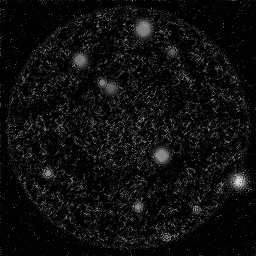
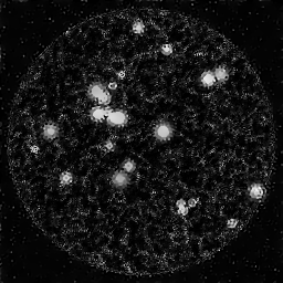
Fiber bundle endoscopy transmits images through a coherent fiber bundle of 10,000-50,000 individual optical fibers. Each fiber core acts as a spatial sample, producing a honeycomb pattern. Image quality is limited by inter-core spacing (pixelation), inter-core coupling (crosstalk), and core-to-core transmission variation. White-light or narrow-band illumination is delivered through the bundle or alongside it. Reconstruction involves core localization, transmission calibration, interpolation to a regular grid, and denoising.
Principle
Fiber-bundle endoscopy transmits an image through a flexible coherent fiber bundle (10,000-100,000 individual fiber cores) to visualize internal body cavities. Each fiber core acts as a single pixel, transmitting light from the distal end to the proximal end where a camera captures the image. The hexagonal fiber packing imposes a fixed pixelation pattern (comb/honeycomb structure) on the image.
How to Build the System
A medical endoscope has a flexible insertion tube containing the coherent fiber bundle (or a distal CMOS chip for video endoscopes), illumination fibers, working channels, and air/water channels. Light source: LED or Xenon lamp transmitted through illumination fibers. For fiber-bundle type: attach a high-resolution camera and relay lens at the proximal end. Calibrate fiber core positions and individual fiber transmission for computational image improvement.
Common Reconstruction Algorithms
- Fiber core mapping and interpolation (honeycomb artifact removal)
- Deep-learning super-resolution for fiber-bundle images
- Structure-from-motion for endoscopic 3-D reconstruction
- Defogging / dehazing for underwater or smoke-obscured endoscopy
- Real-time mosaicking for extended field-of-view endoscopy
Common Mistakes
- Honeycomb pattern artifact from fiber core spacing not removed
- Broken fibers (dark spots) accumulating over time and degrading image quality
- Specular reflections (glare) from wet tissue surfaces saturating the image
- Insufficient illumination causing noisy images in deep body cavities
- Image distortion from fiber bundle bending not corrected
How to Avoid Mistakes
- Apply fiber core interpolation or deep-learning super-resolution in post-processing
- Replace fiber bundles when broken fiber percentage exceeds acceptable threshold
- Use polarization filtering or computational specular removal algorithms
- Use bright LED sources and adjust exposure/gain for adequate signal
- Calibrate and correct for bending-dependent distortion using test patterns
Forward-Model Mismatch Cases
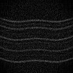
- The widefield fallback produces a (64,64) image, but fiber-bundle endoscopy transmits images through discrete fiber cores creating a hexagonal pixelation pattern — output shape (n_fibers,) is a 1D vector of per-core intensities
- The fiber bundle imposes a fixed sampling grid (honeycomb structure) with inter-core crosstalk and dead fibers — the widefield continuous Gaussian blur has no relationship to the discrete fiber sampling and transmission physics
How to Correct the Mismatch
- Use the endoscopy operator that models per-fiber-core sampling: each of the ~10,000-100,000 cores transmits a point sample from the distal end to the proximal camera, with known core positions and transmission coefficients
- Reconstruct using fiber-core interpolation, honeycomb artifact removal, or deep-learning super-resolution that account for the known fiber bundle geometry and per-core response
Experimental Setup — Signal Chain

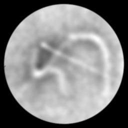
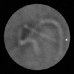
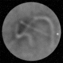
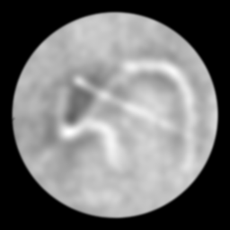
Reconstruction Gallery — 4 Scenes × 3 Scenarios
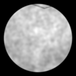
Method: CPU_baseline | Mismatch: nominal (nominal=True, perturbed=False)
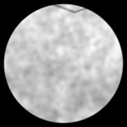
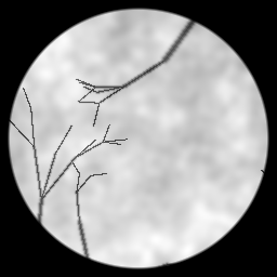
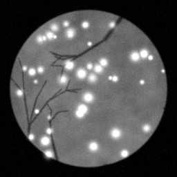
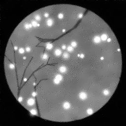
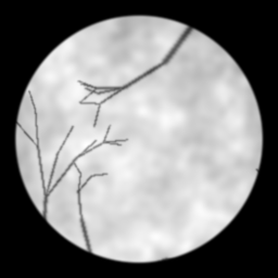
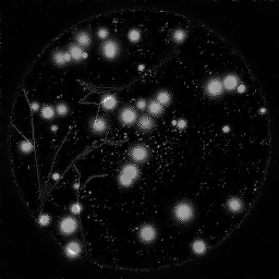
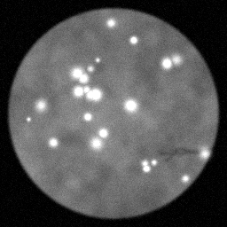
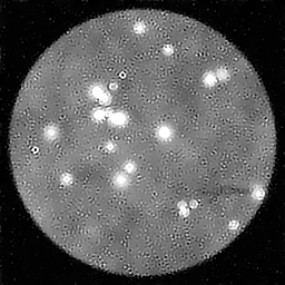
Ground Truth
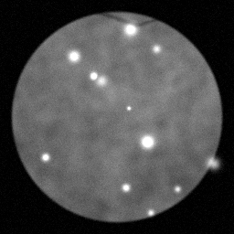
Measurement
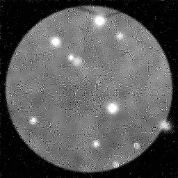
Reconstruction
Ground Truth
Measurement
Reconstruction
Ground Truth
Measurement (perturbed)
Reconstruction


Mean PSNR Across All Scenes
Per-scene PSNR breakdown (4 scenes)
| Scene | I (PSNR) | I (SSIM) | II (PSNR) | II (SSIM) | III (PSNR) | III (SSIM) |
|---|---|---|---|---|---|---|
| scene_00 | 11.330523020774931 | 0.23911573648378578 | 4.34818277975595 | 0.10449569268381598 | 0.0 | 0.0 |
| scene_01 | 11.15564073038409 | 0.48527822586842434 | 3.9899921323310137 | 0.12929610874142025 | 0.0 | 0.0 |
| scene_02 | 11.184935634669307 | 0.22663818537351443 | 5.412581199172374 | 0.07516704036765191 | 0.0 | 0.0 |
| scene_03 | 11.911148737371796 | 0.2887284555129891 | 4.809282504759401 | 0.07142357195974953 | 0.0 | 0.0 |
| Mean | 11.395562030800031 | 0.3099401508096784 | 4.640009654004684 | 0.09509560343815941 | 0.0 | 0.0 |
Experimental Setup
Key References
- Lee & Bhatt, 'Fiber bundle endoscopy advances', J. Biophotonics 12, e201900004 (2019)
Canonical Datasets
- Kvasir-SEG (polyp segmentation)
- CVC-ClinicDB (colonoscopy)
- HyperKvasir (multi-class GI dataset)
Spec DAG — Forward Model Pipeline
C(PSF_fiber) → D(g, η₁)
Mismatch Parameters
| Symbol | Parameter | Description | Nominal | Perturbed |
|---|---|---|---|---|
| Δη_f | fiber_coupling | Fiber coupling efficiency error (%) | 0 | 5.0 |
| Δd | core_spacing | Core spacing error (μm) | 0 | 0.5 |
| Δα_b | bending_loss | Bending loss error (dB) | 0 | 0.3 |
Credits System
Spec Primitives Reference (11 primitives)
Free-space or medium propagation kernel (Fresnel, Rayleigh-Sommerfeld).
Spatial or spatio-temporal amplitude modulation (coded aperture, SLM pattern).
Geometric projection operator (Radon transform, fan-beam, cone-beam).
Sampling in the Fourier / k-space domain (MRI, ptychography).
Shift-invariant convolution with a point-spread function (PSF).
Summation along a physical dimension (spectral, temporal, angular).
Sensor readout with gain g and noise model η (Gaussian, Poisson, mixed).
Patterned illumination (block, Hadamard, random) applied to the scene.
Spectral dispersion element (prism, grating) with shift α and aperture a.
Sample or gantry rotation (CT, electron tomography).
Spectral filter or monochromator selecting a wavelength band.