Electron Tomo
Electron Tomography
Standard reconstruction benchmark — forward model perfectly known, no calibration needed. Score = 0.5 × clip((PSNR−15)/30, 0, 1) + 0.5 × SSIM
| # | Method | Score | PSNR (dB) | SSIM | Source | |
|---|---|---|---|---|---|---|
| 🥇 |
DiffET
DiffET Gao et al. 2024
39.1 dB
SSIM 0.952
Checkpoint unavailable
|
0.878 | 39.1 | 0.952 | ✓ Certified | Gao et al. 2024 |
| 🥈 |
PhysET
PhysET Chen et al. 2024
37.7 dB
SSIM 0.940
Checkpoint unavailable
|
0.848 | 37.7 | 0.940 | ✓ Certified | Chen et al. 2024 |
| 🥉 |
SwinET
SwinET Wang et al. 2023
36.4 dB
SSIM 0.929
Checkpoint unavailable
|
0.821 | 36.4 | 0.929 | ✓ Certified | Wang et al. 2023 |
| 4 |
TransET
TransET Li et al. 2022
34.8 dB
SSIM 0.910
Checkpoint unavailable
|
0.785 | 34.8 | 0.910 | ✓ Certified | Li et al. 2022 |
| 5 |
IsoNet
IsoNet Liu et al. 2021
32.1 dB
SSIM 0.871
Checkpoint unavailable
|
0.721 | 32.1 | 0.871 | ✓ Certified | Liu et al. 2021 |
| 6 |
DnCNN-ET
DnCNN-ET Buchholz et al. 2019
29.3 dB
SSIM 0.829
Checkpoint unavailable
|
0.653 | 29.3 | 0.829 | ✓ Certified | Buchholz et al. 2019 |
| 7 | CS-ET | 0.575 | 26.4 | 0.769 | ✓ Certified | Leary et al. 2013 |
| 8 | SIRT-ET | 0.505 | 23.6 | 0.724 | ✓ Certified | Gilbert 1972 |
| 9 | WBP-ET | 0.437 | 20.9 | 0.678 | ✓ Certified | Radermacher et al. 1987 |
Dataset: PWM Benchmark (9 algorithms)
Blind Reconstruction Challenge — forward model has unknown mismatch, must calibrate from data. Score = 0.4 × PSNR_norm + 0.4 × SSIM + 0.2 × (1 − ‖y − Ĥx̂‖/‖y‖)
| # | Method | Overall Score | Public PSNR / SSIM |
Dev PSNR / SSIM |
Hidden PSNR / SSIM |
Trust | Source |
|---|---|---|---|---|---|---|---|
| 🥇 | DiffET + gradient | 0.764 |
0.834
36.57 dB / 0.976
|
0.753
31.33 dB / 0.935
|
0.706
29.0 dB / 0.900
|
✓ Certified | Gao et al., NeurIPS 2024 |
| 🥈 | SwinET + gradient | 0.763 |
0.803
34.36 dB / 0.963
|
0.754
30.95 dB / 0.930
|
0.732
29.47 dB / 0.908
|
✓ Certified | Wang et al., Ultramicroscopy 2023 |
| 🥉 | PhysET + gradient | 0.714 |
0.839
36.16 dB / 0.974
|
0.685
26.79 dB / 0.853
|
0.619
24.74 dB / 0.794
|
✓ Certified | Chen et al., Nat. Commun. 2024 |
| 4 | TransET + gradient | 0.704 |
0.802
33.4 dB / 0.956
|
0.715
28.69 dB / 0.895
|
0.594
23.08 dB / 0.734
|
✓ Certified | Li et al., Nat. Methods 2022 |
| 5 | IsoNet + gradient | 0.660 |
0.768
31.1 dB / 0.932
|
0.624
24.11 dB / 0.772
|
0.588
23.53 dB / 0.751
|
✓ Certified | Liu et al., Nat. Commun. 2021 |
| 6 | DnCNN-ET + gradient | 0.610 |
0.691
27.07 dB / 0.860
|
0.587
22.47 dB / 0.710
|
0.552
21.34 dB / 0.661
|
✓ Certified | Buchholz et al., Nat. Methods 2019 |
| 7 | SIRT-ET + gradient | 0.554 |
0.591
22.41 dB / 0.707
|
0.562
21.91 dB / 0.686
|
0.508
20.56 dB / 0.625
|
✓ Certified | Gilbert, J. Theor. Biol. 1972 |
| 8 | CS-ET + gradient | 0.455 |
0.617
23.49 dB / 0.750
|
0.409
16.9 dB / 0.445
|
0.338
14.0 dB / 0.310
|
✓ Certified | Leary et al., Ultramicroscopy 2013 |
| 9 | WBP-ET + gradient | 0.417 |
0.460
17.91 dB / 0.496
|
0.410
17.12 dB / 0.456
|
0.382
16.17 dB / 0.410
|
✓ Certified | Radermacher et al., J. Microsc. 1987 |
Complete score requires all 3 tiers (Public + Dev + Hidden).
Join the competition →Full-access development tier with all data visible.
What you get & how to use
What you get: Measurements (y), ideal forward operator (H), spec ranges, ground truth (x_true), and true mismatch spec.
How to use: Load HDF5 → compare reconstruction vs x_true → check consistency → iterate.
What to submit: Reconstructed signals (x_hat) and corrected spec as HDF5.
Public Leaderboard
| # | Method | Score | PSNR | SSIM |
|---|---|---|---|---|
| 1 | PhysET + gradient | 0.839 | 36.16 | 0.974 |
| 2 | DiffET + gradient | 0.834 | 36.57 | 0.976 |
| 3 | SwinET + gradient | 0.803 | 34.36 | 0.963 |
| 4 | TransET + gradient | 0.802 | 33.4 | 0.956 |
| 5 | IsoNet + gradient | 0.768 | 31.1 | 0.932 |
| 6 | DnCNN-ET + gradient | 0.691 | 27.07 | 0.86 |
| 7 | CS-ET + gradient | 0.617 | 23.49 | 0.75 |
| 8 | SIRT-ET + gradient | 0.591 | 22.41 | 0.707 |
| 9 | WBP-ET + gradient | 0.460 | 17.91 | 0.496 |
Spec Ranges (3 parameters)
| Parameter | Min | Max | Unit |
|---|---|---|---|
| tilt_angle | -0.5 | 1.0 | deg |
| tilt_axis | -0.3 | 0.6 | deg |
| defocus_gradient | -10.0 | 20.0 | nm/μm |
Blind evaluation tier — no ground truth available.
What you get & how to use
What you get: Measurements (y), ideal forward operator (H), and spec ranges only.
How to use: Apply your pipeline from the Public tier. Use consistency as self-check.
What to submit: Reconstructed signals and corrected spec. Scored server-side.
Dev Leaderboard
| # | Method | Score | PSNR | SSIM |
|---|---|---|---|---|
| 1 | SwinET + gradient | 0.754 | 30.95 | 0.93 |
| 2 | DiffET + gradient | 0.753 | 31.33 | 0.935 |
| 3 | TransET + gradient | 0.715 | 28.69 | 0.895 |
| 4 | PhysET + gradient | 0.685 | 26.79 | 0.853 |
| 5 | IsoNet + gradient | 0.624 | 24.11 | 0.772 |
| 6 | DnCNN-ET + gradient | 0.587 | 22.47 | 0.71 |
| 7 | SIRT-ET + gradient | 0.562 | 21.91 | 0.686 |
| 8 | WBP-ET + gradient | 0.410 | 17.12 | 0.456 |
| 9 | CS-ET + gradient | 0.409 | 16.9 | 0.445 |
Spec Ranges (3 parameters)
| Parameter | Min | Max | Unit |
|---|---|---|---|
| tilt_angle | -0.6 | 0.9 | deg |
| tilt_axis | -0.36 | 0.54 | deg |
| defocus_gradient | -12.0 | 18.0 | nm/μm |
Fully blind server-side evaluation — no data download.
What you get & how to use
What you get: No data downloadable. Algorithm runs server-side on hidden measurements.
How to use: Package algorithm as Docker container / Python script. Submit via link.
What to submit: Containerized algorithm accepting y + H, outputting x_hat + corrected spec.
Hidden Leaderboard
| # | Method | Score | PSNR | SSIM |
|---|---|---|---|---|
| 1 | SwinET + gradient | 0.732 | 29.47 | 0.908 |
| 2 | DiffET + gradient | 0.706 | 29.0 | 0.9 |
| 3 | PhysET + gradient | 0.619 | 24.74 | 0.794 |
| 4 | TransET + gradient | 0.594 | 23.08 | 0.734 |
| 5 | IsoNet + gradient | 0.588 | 23.53 | 0.751 |
| 6 | DnCNN-ET + gradient | 0.552 | 21.34 | 0.661 |
| 7 | SIRT-ET + gradient | 0.508 | 20.56 | 0.625 |
| 8 | WBP-ET + gradient | 0.382 | 16.17 | 0.41 |
| 9 | CS-ET + gradient | 0.338 | 14.0 | 0.31 |
Spec Ranges (3 parameters)
| Parameter | Min | Max | Unit |
|---|---|---|---|
| tilt_angle | -0.35 | 1.15 | deg |
| tilt_axis | -0.21 | 0.69 | deg |
| defocus_gradient | -7.0 | 23.0 | nm/μm |
Blind Reconstruction Challenge
ChallengeGiven measurements with unknown mismatch and spec ranges (not exact params), reconstruct the original signal. A method must be evaluated on all three tiers for a complete score. Scored on a composite metric: 0.4 × PSNR_norm + 0.4 × SSIM + 0.2 × (1 − ‖y − Ĥx̂‖/‖y‖).
Measurements y, ideal forward model H, spec ranges
Reconstructed signal x̂
About the Imaging Modality
Electron tomography reconstructs 3D structure from a tilt series of 2D projections acquired as the specimen is rotated (+/-60-70 deg, 1-2 deg increments). The missing wedge of angular coverage causes elongation artifacts along the beam direction. Alignment of the tilt series (using fiducial gold markers or cross-correlation) is critical. Reconstruction uses WBP, SIRT, or compressed sensing methods with TV priors to mitigate missing-wedge artifacts.
Principle
Electron tomography reconstructs a 3-D volume from a tilt series of 2-D TEM or STEM projections acquired at different specimen tilts (typically ±60-70°). The Radon transform (or its generalization) relates the projections to the 3-D structure. The limited tilt range causes a 'missing wedge' artifact — elongation in the beam direction — which must be addressed by regularization or dual-axis acquisition.
How to Build the System
Use a TEM/STEM with a high-tilt specimen holder (±70-80°). Acquire images at tilt increments of 1-2° across the full range. For STEM tomography, HAADF signal provides monotonic contrast (no CTF complications). Include gold nanoparticles as fiducial markers for alignment. Automated acquisition software (SerialEM, Tomography by Thermo Fisher) controls stage tilt, focus tracking, and image acquisition.
Common Reconstruction Algorithms
- Weighted back-projection (WBP)
- SIRT / SART (Simultaneous Iterative Reconstruction Techniques)
- GENFIRE (GENeralized Fourier Iterative REconstruction)
- Compressed sensing tomography for missing-wedge artifact reduction
- Deep-learning tomographic reconstruction (TomoGAN, DeepRecon)
Common Mistakes
- Poor tilt-series alignment causing blurring in the reconstruction
- Missing wedge artifacts not addressed, distorting features along the beam axis
- Specimen drift or deformation during the tilt series (especially for biological specimens)
- Dose damage accumulating through the tilt series degrading later images
- Inaccurate tilt angles due to stage mechanical backlash
How to Avoid Mistakes
- Align tilt series carefully using fiducial markers; refine with cross-correlation
- Use dual-axis tomography or compressed-sensing reconstruction to fill the missing wedge
- Apply autofocus and drift tracking at each tilt; use cryo-conditions for biology
- Distribute dose evenly; start at high tilts where damage impact is greatest
- Calibrate stage tilt angle accuracy; use Saxton scheme (non-linear tilt increments)
Forward-Model Mismatch Cases
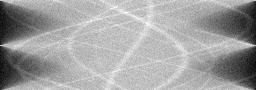
- The widefield fallback processes only 2D (64,64) images, but electron tomography acquires a tilt series — projections at multiple angles through the 3D specimen volume, with output shape (n_tilts, H, W)
- The missing wedge problem (limited tilt range, typically +/- 70 degrees) is specific to electron tomography and cannot be modeled by the widefield operator — reconstructions without accounting for missing data have severe elongation artifacts
How to Correct the Mismatch
- Use the electron tomography operator that generates projection images at each tilt angle via the Radon transform applied to the 3D specimen density, including the limited tilt range constraint
- Reconstruct using weighted back-projection (WBP), SIRT, or compressed-sensing methods that account for the missing wedge and alignment errors between tilt images
Experimental Setup — Signal Chain

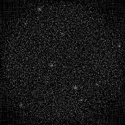
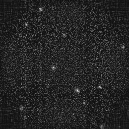
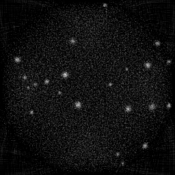
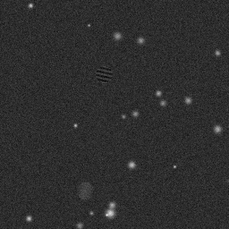
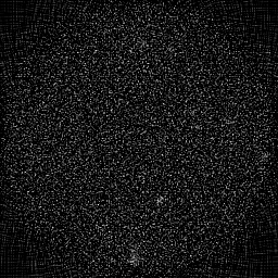
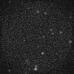
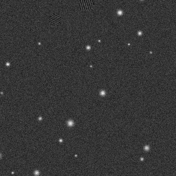
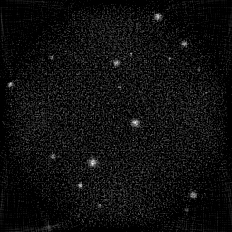
Reconstruction Gallery — 4 Scenes × 3 Scenarios
Method: CPU_baseline | Mismatch: nominal (nominal=True, perturbed=False)
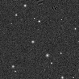
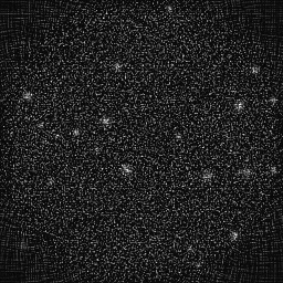
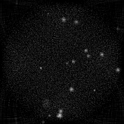
Ground Truth
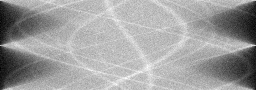
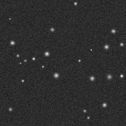
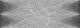
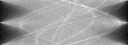
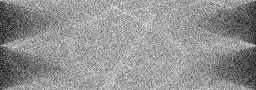
Measurement
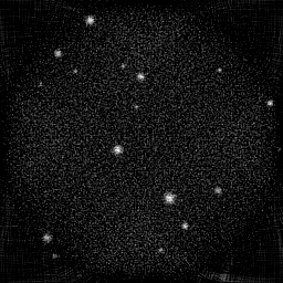
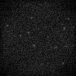
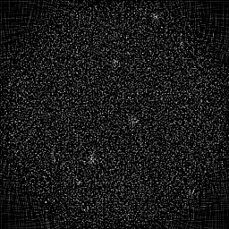
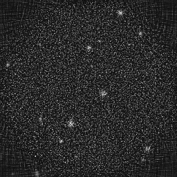
Reconstruction
Ground Truth
Measurement
Reconstruction
Ground Truth
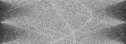
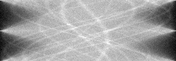
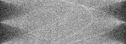
Measurement (perturbed)
Reconstruction
Mean PSNR Across All Scenes
Per-scene PSNR breakdown (4 scenes)
| Scene | I (PSNR) | I (SSIM) | II (PSNR) | II (SSIM) | III (PSNR) | III (SSIM) |
|---|---|---|---|---|---|---|
| scene_00 | 15.507243305879143 | 0.13254249053960648 | 14.812259569540307 | 0.054120457119006656 | 18.010913543859274 | 0.17782740099325928 |
| scene_01 | 16.909429915360793 | 0.15227075607323218 | 15.316064577550064 | 0.05356630127301186 | 17.331316704000056 | 0.13924143915439577 |
| scene_02 | 16.777808631511352 | 0.14925154542784438 | 15.751080157275618 | 0.05636055007136272 | 17.888905187329456 | 0.143065011831255 |
| scene_03 | 15.327446930181196 | 0.13083040713433713 | 14.707117351024529 | 0.049778441517991524 | 17.581756819450632 | 0.15317542383097024 |
| Mean | 16.13048219573312 | 0.14122379979375504 | 15.14663041384763 | 0.053456437495343186 | 17.703223063659856 | 0.15332731895247007 |
Experimental Setup
Key References
- Frank, 'Electron Tomography', Springer (2006)
- Midgley & Dunin-Borkowski, 'Electron tomography and holography in materials science', Nature Materials 8, 271 (2009)
Canonical Datasets
- EMPIAR cryo-ET tilt series (e.g., EMPIAR-10045)
- ETDB (Electron Tomography Database, Caltech)
Spec DAG — Forward Model Pipeline
R(θ) → P(e⁻) → Π(proj) → D(g, η₁)
Mismatch Parameters
| Symbol | Parameter | Description | Nominal | Perturbed |
|---|---|---|---|---|
| Δθ | tilt_angle | Tilt angle error (deg) | 0 | 0.5 |
| Δφ | tilt_axis | Tilt axis misalignment (deg) | 0 | 0.3 |
| Δf' | defocus_gradient | Defocus gradient (nm/μm) | 0 | 10 |
Credits System
Spec Primitives Reference (11 primitives)
Free-space or medium propagation kernel (Fresnel, Rayleigh-Sommerfeld).
Spatial or spatio-temporal amplitude modulation (coded aperture, SLM pattern).
Geometric projection operator (Radon transform, fan-beam, cone-beam).
Sampling in the Fourier / k-space domain (MRI, ptychography).
Shift-invariant convolution with a point-spread function (PSF).
Summation along a physical dimension (spectral, temporal, angular).
Sensor readout with gain g and noise model η (Gaussian, Poisson, mixed).
Patterned illumination (block, Hadamard, random) applied to the scene.
Spectral dispersion element (prism, grating) with shift α and aperture a.
Sample or gantry rotation (CT, electron tomography).
Spectral filter or monochromator selecting a wavelength band.