4D-STEM
4D-STEM Electron Diffraction
Standard reconstruction benchmark — forward model perfectly known, no calibration needed. Score = 0.5 × clip((PSNR−15)/30, 0, 1) + 0.5 × SSIM
| # | Method | Score | PSNR (dB) | SSIM | Source | |
|---|---|---|---|---|---|---|
| 🥇 |
DiffED
DiffED Gao et al. 2024
39.1 dB
SSIM 0.953
Checkpoint unavailable
|
0.878 | 39.1 | 0.953 | ✓ Certified | Gao et al. 2024 |
| 🥈 |
PhysED
PhysED Chen et al. 2024
37.7 dB
SSIM 0.941
Checkpoint unavailable
|
0.849 | 37.7 | 0.941 | ✓ Certified | Chen et al. 2024 |
| 🥉 |
SwinED
SwinED Wang et al. 2023
36.4 dB
SSIM 0.930
Checkpoint unavailable
|
0.822 | 36.4 | 0.930 | ✓ Certified | Wang et al. 2023 |
| 4 |
TransED
TransED Li et al. 2022
34.8 dB
SSIM 0.912
Checkpoint unavailable
|
0.786 | 34.8 | 0.912 | ✓ Certified | Li et al. 2022 |
| 5 | PhaseGAN-ED | 0.725 | 32.3 | 0.873 | ✓ Certified | Zimmermann et al. 2021 |
| 6 |
DnCNN-ED
DnCNN-ED Cherukara et al. 2018
29.5 dB
SSIM 0.833
Checkpoint unavailable
|
0.658 | 29.5 | 0.833 | ✓ Certified | Cherukara et al. 2018 |
| 7 | MicroED | 0.586 | 26.7 | 0.781 | ✓ Certified | Shi et al. 2013 |
| 8 | PEDT | 0.517 | 23.9 | 0.738 | ✓ Certified | Kolb et al. 2007 |
| 9 | Direct-Methods | 0.450 | 21.2 | 0.694 | ✓ Certified | Hauptman & Karle 1985 |
Dataset: PWM Benchmark (9 algorithms)
Blind Reconstruction Challenge — forward model has unknown mismatch, must calibrate from data. Score = 0.4 × PSNR_norm + 0.4 × SSIM + 0.2 × (1 − ‖y − Ĥx̂‖/‖y‖)
| # | Method | Overall Score | Public PSNR / SSIM |
Dev PSNR / SSIM |
Hidden PSNR / SSIM |
Trust | Source |
|---|---|---|---|---|---|---|---|
| 🥇 | DiffED + gradient | 0.767 |
0.837
36.95 dB / 0.978
|
0.742
31.09 dB / 0.932
|
0.723
29.78 dB / 0.913
|
✓ Certified | Gao et al., NeurIPS 2024 |
| 🥈 | PhysED + gradient | 0.752 |
0.839
36.32 dB / 0.975
|
0.732
30.43 dB / 0.923
|
0.684
27.13 dB / 0.861
|
✓ Certified | Chen et al., Nat. Commun. 2024 |
| 🥉 | SwinED + gradient | 0.747 |
0.801
33.87 dB / 0.960
|
0.755
30.61 dB / 0.926
|
0.684
27.17 dB / 0.862
|
✓ Certified | Wang et al., npj Comput. Mater. 2023 |
| 4 | TransED + gradient | 0.702 |
0.780
32.33 dB / 0.946
|
0.713
28.13 dB / 0.883
|
0.612
23.77 dB / 0.760
|
✓ Certified | Li et al., Nat. Commun. 2022 |
| 5 | PhaseGAN-ED + gradient | 0.641 |
0.767
30.77 dB / 0.928
|
0.621
24.33 dB / 0.780
|
0.536
20.8 dB / 0.636
|
✓ Certified | Zimmermann et al., Sci. Adv. 2021 |
| 6 | MicroED + gradient | 0.617 |
0.641
24.91 dB / 0.799
|
0.609
23.56 dB / 0.753
|
0.602
24.04 dB / 0.770
|
✓ Certified | Shi et al., eLife 2013 |
| 7 | DnCNN-ED + gradient | 0.558 |
0.721
28.14 dB / 0.884
|
0.522
20.29 dB / 0.613
|
0.430
17.91 dB / 0.496
|
✓ Certified | Cherukara et al., npj Comput. Mater. 2018 |
| 8 | PEDT + gradient | 0.511 |
0.566
21.76 dB / 0.680
|
0.512
20.43 dB / 0.619
|
0.456
18.92 dB / 0.546
|
✓ Certified | Kolb et al., Ultramicroscopy 2007 |
| 9 | Direct-Methods + gradient | 0.470 |
0.518
19.67 dB / 0.583
|
0.454
18.46 dB / 0.523
|
0.437
17.37 dB / 0.469
|
✓ Certified | Hauptman & Karle, Nobel Prize 1985 |
Complete score requires all 3 tiers (Public + Dev + Hidden).
Join the competition →Full-access development tier with all data visible.
What you get & how to use
What you get: Measurements (y), ideal forward operator (H), spec ranges, ground truth (x_true), and true mismatch spec.
How to use: Load HDF5 → compare reconstruction vs x_true → check consistency → iterate.
What to submit: Reconstructed signals (x_hat) and corrected spec as HDF5.
Public Leaderboard
| # | Method | Score | PSNR | SSIM |
|---|---|---|---|---|
| 1 | PhysED + gradient | 0.839 | 36.32 | 0.975 |
| 2 | DiffED + gradient | 0.837 | 36.95 | 0.978 |
| 3 | SwinED + gradient | 0.801 | 33.87 | 0.96 |
| 4 | TransED + gradient | 0.780 | 32.33 | 0.946 |
| 5 | PhaseGAN-ED + gradient | 0.767 | 30.77 | 0.928 |
| 6 | DnCNN-ED + gradient | 0.721 | 28.14 | 0.884 |
| 7 | MicroED + gradient | 0.641 | 24.91 | 0.799 |
| 8 | PEDT + gradient | 0.566 | 21.76 | 0.68 |
| 9 | Direct-Methods + gradient | 0.518 | 19.67 | 0.583 |
Spec Ranges (3 parameters)
| Parameter | Min | Max | Unit |
|---|---|---|---|
| camera_length | -2.0 | 4.0 | % |
| center_offset | -1.0 | 2.0 | pixels |
| elliptical_distortion | -0.005 | 0.01 |
Blind evaluation tier — no ground truth available.
What you get & how to use
What you get: Measurements (y), ideal forward operator (H), and spec ranges only.
How to use: Apply your pipeline from the Public tier. Use consistency as self-check.
What to submit: Reconstructed signals and corrected spec. Scored server-side.
Dev Leaderboard
| # | Method | Score | PSNR | SSIM |
|---|---|---|---|---|
| 1 | SwinED + gradient | 0.755 | 30.61 | 0.926 |
| 2 | DiffED + gradient | 0.742 | 31.09 | 0.932 |
| 3 | PhysED + gradient | 0.732 | 30.43 | 0.923 |
| 4 | TransED + gradient | 0.713 | 28.13 | 0.883 |
| 5 | PhaseGAN-ED + gradient | 0.621 | 24.33 | 0.78 |
| 6 | MicroED + gradient | 0.609 | 23.56 | 0.753 |
| 7 | DnCNN-ED + gradient | 0.522 | 20.29 | 0.613 |
| 8 | PEDT + gradient | 0.512 | 20.43 | 0.619 |
| 9 | Direct-Methods + gradient | 0.454 | 18.46 | 0.523 |
Spec Ranges (3 parameters)
| Parameter | Min | Max | Unit |
|---|---|---|---|
| camera_length | -2.4 | 3.6 | % |
| center_offset | -1.2 | 1.8 | pixels |
| elliptical_distortion | -0.006 | 0.009 |
Fully blind server-side evaluation — no data download.
What you get & how to use
What you get: No data downloadable. Algorithm runs server-side on hidden measurements.
How to use: Package algorithm as Docker container / Python script. Submit via link.
What to submit: Containerized algorithm accepting y + H, outputting x_hat + corrected spec.
Hidden Leaderboard
| # | Method | Score | PSNR | SSIM |
|---|---|---|---|---|
| 1 | DiffED + gradient | 0.723 | 29.78 | 0.913 |
| 2 | PhysED + gradient | 0.684 | 27.13 | 0.861 |
| 3 | SwinED + gradient | 0.684 | 27.17 | 0.862 |
| 4 | TransED + gradient | 0.612 | 23.77 | 0.76 |
| 5 | MicroED + gradient | 0.602 | 24.04 | 0.77 |
| 6 | PhaseGAN-ED + gradient | 0.536 | 20.8 | 0.636 |
| 7 | PEDT + gradient | 0.456 | 18.92 | 0.546 |
| 8 | Direct-Methods + gradient | 0.437 | 17.37 | 0.469 |
| 9 | DnCNN-ED + gradient | 0.430 | 17.91 | 0.496 |
Spec Ranges (3 parameters)
| Parameter | Min | Max | Unit |
|---|---|---|---|
| camera_length | -1.4 | 4.6 | % |
| center_offset | -0.7 | 2.3 | pixels |
| elliptical_distortion | -0.0035 | 0.0115 |
Blind Reconstruction Challenge
ChallengeGiven measurements with unknown mismatch and spec ranges (not exact params), reconstruct the original signal. A method must be evaluated on all three tiers for a complete score. Scored on a composite metric: 0.4 × PSNR_norm + 0.4 × SSIM + 0.2 × (1 − ‖y − Ĥx̂‖/‖y‖).
Measurements y, ideal forward model H, spec ranges
Reconstructed signal x̂
About the Imaging Modality
4D-STEM acquires a full 2D convergent-beam electron diffraction (CBED) pattern at each probe position during a 2D STEM scan, yielding a 4D dataset (2 real-space + 2 reciprocal-space dimensions). This enables simultaneous mapping of strain, orientation, electric fields, and thickness with nanometer spatial resolution. Phase retrieval from the 4D dataset (electron ptychography) can achieve sub-angstrom resolution. High data rates (>1 GB/s) from fast pixelated detectors create computational challenges.
Principle
4D-STEM electron diffraction scans a convergent electron beam across the specimen and records a full 2-D diffraction pattern (convergent beam electron diffraction, CBED) at each scan position. The resulting 4-D dataset (2-D scan × 2-D diffraction) enables mapping of crystal structure, orientation, strain, electric fields, and charge density with nanometer spatial resolution.
How to Build the System
Use a STEM equipped with a fast pixelated detector (Medipix3, EMPAD, or Dectris ARINA) capable of recording diffraction patterns at >1000 fps. Set a small convergence semi-angle (1-5 mrad) for nanobeam diffraction or large (20-30 mrad) for CBED. The scan step should be comparable to the probe size. Data volumes are large (tens of GB per scan), requiring efficient data pipeline and storage.
Common Reconstruction Algorithms
- Virtual detector imaging (synthesized BF, DF, iDPC from 4D data)
- Center-of-mass (COM) analysis for electric field mapping
- Ptychographic reconstruction from 4D-STEM data
- Orientation mapping (template matching against simulated patterns)
- Strain mapping via disk position analysis
Common Mistakes
- Detector dynamic range insufficient for simultaneous central beam and weak diffraction
- Scan step too large relative to probe size, under-sampling the specimen
- Not accounting for specimen thickness variation in diffraction pattern interpretation
- Excessive electron dose for beam-sensitive materials (organics, 2D materials)
- Misindexing diffraction patterns due to double diffraction or overlapping grains
How to Avoid Mistakes
- Use counting-mode detectors (Medipix) with high dynamic range or electron counting
- Match scan step to probe size for complete spatial sampling
- Simulate diffraction patterns at the measured thickness for accurate interpretation
- Use low-dose 4D-STEM protocols with fast detectors to minimize beam damage
- Carefully index patterns considering multiple scattering; compare with simulations
Forward-Model Mismatch Cases
- The widefield fallback produces a real-space blurred image, but electron diffraction records the far-field diffraction pattern (reciprocal space) — Bragg spots encode crystal structure, lattice spacings, and symmetry, which bear no resemblance to a blurred image
- The diffraction pattern intensity I(k) = |F{V(r) * P(r)}|^2 encodes the Fourier transform of the projected crystal potential — the widefield real-space blur cannot access reciprocal-space crystallographic information
How to Correct the Mismatch
- Use the electron diffraction operator that models kinematic or dynamical scattering from the crystal lattice, producing far-field diffraction patterns with Bragg peaks at reciprocal lattice positions
- Index diffraction patterns to determine crystal structure and orientation; use dynamical simulation (Bloch wave or multislice) for accurate intensity matching and structure refinement
Experimental Setup — Signal Chain

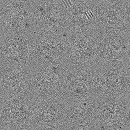
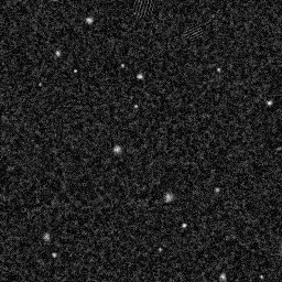
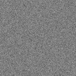
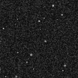
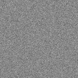
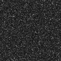
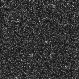
Reconstruction Gallery — 4 Scenes × 3 Scenarios
Method: CPU_baseline | Mismatch: nominal (nominal=True, perturbed=False)
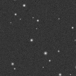
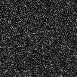
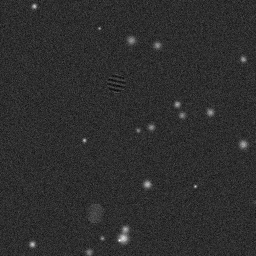
Ground Truth
Measurement
Reconstruction
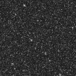
Ground Truth
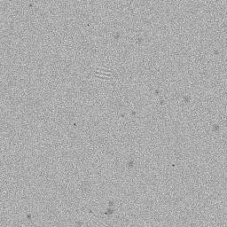
Measurement
Reconstruction
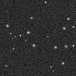
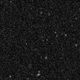
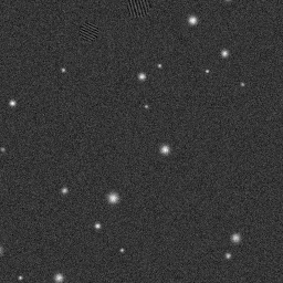
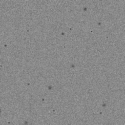
Ground Truth
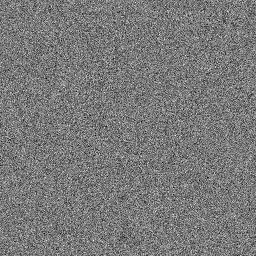
Measurement (perturbed)
Reconstruction
Mean PSNR Across All Scenes
Per-scene PSNR breakdown (4 scenes)
| Scene | I (PSNR) | I (SSIM) | II (PSNR) | II (SSIM) | III (PSNR) | III (SSIM) |
|---|---|---|---|---|---|---|
| scene_00 | 19.401488157362497 | 0.48886704895877836 | 16.857966791337656 | 0.08915507096515726 | 19.015339082048712 | 0.19323876033569679 |
| scene_01 | 20.386994971632934 | 0.49771035050842166 | 17.188182006293506 | 0.08456095595654231 | 19.00326347865052 | 0.1825080566719887 |
| scene_02 | 20.109288125342772 | 0.4612187812713385 | 17.552917796407378 | 0.08129459333217216 | 19.721316784917846 | 0.17921822573660165 |
| scene_03 | 19.33896725172696 | 0.48831334454774855 | 16.902556624008536 | 0.09105537055754624 | 18.83727554088228 | 0.1898195007747968 |
| Mean | 19.80918462651629 | 0.48402738132157175 | 17.125405804511768 | 0.0865164977028545 | 19.144298721624843 | 0.186196135879771 |
Experimental Setup
Key References
- Ophus, 'Four-dimensional scanning transmission electron microscopy', Microscopy & Microanalysis 25, 563 (2019)
- Jiang et al., 'Electron ptychography of 2D materials to deep sub-angstrom resolution', Nature 559, 343 (2018)
Canonical Datasets
- 4D-STEM benchmark datasets (Ophus group, NCEM)
Spec DAG — Forward Model Pipeline
P(e⁻) → F(diffraction) → D(g, η₁)
Mismatch Parameters
| Symbol | Parameter | Description | Nominal | Perturbed |
|---|---|---|---|---|
| ΔL | camera_length | Camera length error (%) | 0 | 2.0 |
| Δc | center_offset | Diffraction center offset (pixels) | 0 | 1.0 |
| ε | elliptical_distortion | Elliptical distortion | 0 | 0.005 |
Credits System
Spec Primitives Reference (11 primitives)
Free-space or medium propagation kernel (Fresnel, Rayleigh-Sommerfeld).
Spatial or spatio-temporal amplitude modulation (coded aperture, SLM pattern).
Geometric projection operator (Radon transform, fan-beam, cone-beam).
Sampling in the Fourier / k-space domain (MRI, ptychography).
Shift-invariant convolution with a point-spread function (PSF).
Summation along a physical dimension (spectral, temporal, angular).
Sensor readout with gain g and noise model η (Gaussian, Poisson, mixed).
Patterned illumination (block, Hadamard, random) applied to the scene.
Spectral dispersion element (prism, grating) with shift α and aperture a.
Sample or gantry rotation (CT, electron tomography).
Spectral filter or monochromator selecting a wavelength band.