Elastography
Shear-Wave Elastography
Standard reconstruction benchmark — forward model perfectly known, no calibration needed. Score = 0.5 × clip((PSNR−15)/30, 0, 1) + 0.5 × SSIM
| # | Method | Score | PSNR (dB) | SSIM | Source | |
|---|---|---|---|---|---|---|
| 🥇 |
DiffElasto
DiffElasto Gao et al. 2024
39.2 dB
SSIM 0.953
Checkpoint unavailable
|
0.880 | 39.2 | 0.953 | ✓ Certified | Gao et al. 2024 |
| 🥈 |
PhysElasto
PhysElasto Chen et al. 2024
37.8 dB
SSIM 0.942
Checkpoint unavailable
|
0.851 | 37.8 | 0.942 | ✓ Certified | Chen et al. 2024 |
| 🥉 |
SwinElasto
SwinElasto Wang et al. 2023
36.6 dB
SSIM 0.932
Checkpoint unavailable
|
0.826 | 36.6 | 0.932 | ✓ Certified | Wang et al. 2023 |
| 4 |
TransElasto
TransElasto Li et al. 2022
35.0 dB
SSIM 0.915
Checkpoint unavailable
|
0.791 | 35.0 | 0.915 | ✓ Certified | Li et al. 2022 |
| 5 |
ElastoNet
ElastoNet Tzschatzsch et al. 2021
32.5 dB
SSIM 0.876
Checkpoint unavailable
|
0.730 | 32.5 | 0.876 | ✓ Certified | Tzschatzsch et al. 2021 |
| 6 |
DnCNN-Elasto
DnCNN-Elasto Guo et al. 2019
29.7 dB
SSIM 0.838
Checkpoint unavailable
|
0.664 | 29.7 | 0.838 | ✓ Certified | Guo et al. 2019 |
| 7 | AIDE | 0.592 | 26.9 | 0.787 | ✓ Certified | Oliphant et al. 2001 |
| 8 | DI-Elasto | 0.539 | 24.8 | 0.752 | ✓ Certified | Van Houten et al. 2001 |
| 9 | LFE-Elasto | 0.477 | 22.3 | 0.710 | ✓ Certified | Manduca et al. 2001 |
Dataset: PWM Benchmark (9 algorithms)
Blind Reconstruction Challenge — forward model has unknown mismatch, must calibrate from data. Score = 0.4 × PSNR_norm + 0.4 × SSIM + 0.2 × (1 − ‖y − Ĥx̂‖/‖y‖)
| # | Method | Overall Score | Public PSNR / SSIM |
Dev PSNR / SSIM |
Hidden PSNR / SSIM |
Trust | Source |
|---|---|---|---|---|---|---|---|
| 🥇 | DiffElasto + gradient | 0.782 |
0.857
38.02 dB / 0.982
|
0.760
31.26 dB / 0.934
|
0.729
30.49 dB / 0.924
|
✓ Certified | Gao et al., MICCAI 2024 |
| 🥈 | SwinElasto + gradient | 0.773 |
0.828
35.51 dB / 0.971
|
0.760
31.91 dB / 0.942
|
0.730
29.97 dB / 0.916
|
✓ Certified | Wang et al., IEEE TMI 2023 |
| 🥉 | PhysElasto + gradient | 0.762 |
0.841
36.43 dB / 0.976
|
0.750
30.47 dB / 0.924
|
0.694
28.68 dB / 0.894
|
✓ Certified | Chen et al., Magn. Reson. Med. 2024 |
| 4 | TransElasto + gradient | 0.742 |
0.782
32.22 dB / 0.945
|
0.754
31.09 dB / 0.932
|
0.689
28.03 dB / 0.881
|
✓ Certified | Li et al., Magn. Reson. Med. 2022 |
| 5 | ElastoNet + gradient | 0.670 |
0.745
29.99 dB / 0.917
|
0.655
25.36 dB / 0.813
|
0.611
24.5 dB / 0.786
|
✓ Certified | Tzschatzsch et al., IEEE TMI 2021 |
| 6 | DnCNN-Elasto + gradient | 0.587 |
0.693
26.97 dB / 0.857
|
0.546
20.98 dB / 0.645
|
0.522
20.57 dB / 0.626
|
✓ Certified | Guo et al., Med. Phys. 2019 |
| 7 | LFE-Elasto + gradient | 0.498 |
0.516
20.02 dB / 0.600
|
0.490
19.27 dB / 0.563
|
0.488
19.83 dB / 0.590
|
✓ Certified | Manduca et al., Magn. Reson. Imaging 2001 |
| 8 | AIDE + gradient | 0.457 |
0.638
24.6 dB / 0.789
|
0.408
16.26 dB / 0.414
|
0.326
14.28 dB / 0.322
|
✓ Certified | Oliphant et al., Magn. Reson. Med. 2001 |
| 9 | DI-Elasto + gradient | 0.444 |
0.623
23.56 dB / 0.753
|
0.405
16.49 dB / 0.425
|
0.305
13.3 dB / 0.281
|
✓ Certified | Van Houten et al., Magn. Reson. Med. 2001 |
Complete score requires all 3 tiers (Public + Dev + Hidden).
Join the competition →Full-access development tier with all data visible.
What you get & how to use
What you get: Measurements (y), ideal forward operator (H), spec ranges, ground truth (x_true), and true mismatch spec.
How to use: Load HDF5 → compare reconstruction vs x_true → check consistency → iterate.
What to submit: Reconstructed signals (x_hat) and corrected spec as HDF5.
Public Leaderboard
| # | Method | Score | PSNR | SSIM |
|---|---|---|---|---|
| 1 | DiffElasto + gradient | 0.857 | 38.02 | 0.982 |
| 2 | PhysElasto + gradient | 0.841 | 36.43 | 0.976 |
| 3 | SwinElasto + gradient | 0.828 | 35.51 | 0.971 |
| 4 | TransElasto + gradient | 0.782 | 32.22 | 0.945 |
| 5 | ElastoNet + gradient | 0.745 | 29.99 | 0.917 |
| 6 | DnCNN-Elasto + gradient | 0.693 | 26.97 | 0.857 |
| 7 | AIDE + gradient | 0.638 | 24.6 | 0.789 |
| 8 | DI-Elasto + gradient | 0.623 | 23.56 | 0.753 |
| 9 | LFE-Elasto + gradient | 0.516 | 20.02 | 0.6 |
Spec Ranges (3 parameters)
| Parameter | Min | Max | Unit |
|---|---|---|---|
| shear_speed | -0.3 | 0.6 | m/s |
| push_duration | -10.0 | 20.0 | μs |
| tissue_viscosity | -15.0 | 30.0 | % |
Blind evaluation tier — no ground truth available.
What you get & how to use
What you get: Measurements (y), ideal forward operator (H), and spec ranges only.
How to use: Apply your pipeline from the Public tier. Use consistency as self-check.
What to submit: Reconstructed signals and corrected spec. Scored server-side.
Dev Leaderboard
| # | Method | Score | PSNR | SSIM |
|---|---|---|---|---|
| 1 | DiffElasto + gradient | 0.760 | 31.26 | 0.934 |
| 2 | SwinElasto + gradient | 0.760 | 31.91 | 0.942 |
| 3 | TransElasto + gradient | 0.754 | 31.09 | 0.932 |
| 4 | PhysElasto + gradient | 0.750 | 30.47 | 0.924 |
| 5 | ElastoNet + gradient | 0.655 | 25.36 | 0.813 |
| 6 | DnCNN-Elasto + gradient | 0.546 | 20.98 | 0.645 |
| 7 | LFE-Elasto + gradient | 0.490 | 19.27 | 0.563 |
| 8 | AIDE + gradient | 0.408 | 16.26 | 0.414 |
| 9 | DI-Elasto + gradient | 0.405 | 16.49 | 0.425 |
Spec Ranges (3 parameters)
| Parameter | Min | Max | Unit |
|---|---|---|---|
| shear_speed | -0.36 | 0.54 | m/s |
| push_duration | -12.0 | 18.0 | μs |
| tissue_viscosity | -18.0 | 27.0 | % |
Fully blind server-side evaluation — no data download.
What you get & how to use
What you get: No data downloadable. Algorithm runs server-side on hidden measurements.
How to use: Package algorithm as Docker container / Python script. Submit via link.
What to submit: Containerized algorithm accepting y + H, outputting x_hat + corrected spec.
Hidden Leaderboard
| # | Method | Score | PSNR | SSIM |
|---|---|---|---|---|
| 1 | SwinElasto + gradient | 0.730 | 29.97 | 0.916 |
| 2 | DiffElasto + gradient | 0.729 | 30.49 | 0.924 |
| 3 | PhysElasto + gradient | 0.694 | 28.68 | 0.894 |
| 4 | TransElasto + gradient | 0.689 | 28.03 | 0.881 |
| 5 | ElastoNet + gradient | 0.611 | 24.5 | 0.786 |
| 6 | DnCNN-Elasto + gradient | 0.522 | 20.57 | 0.626 |
| 7 | LFE-Elasto + gradient | 0.488 | 19.83 | 0.59 |
| 8 | AIDE + gradient | 0.326 | 14.28 | 0.322 |
| 9 | DI-Elasto + gradient | 0.305 | 13.3 | 0.281 |
Spec Ranges (3 parameters)
| Parameter | Min | Max | Unit |
|---|---|---|---|
| shear_speed | -0.21 | 0.69 | m/s |
| push_duration | -7.0 | 23.0 | μs |
| tissue_viscosity | -10.5 | 34.5 | % |
Blind Reconstruction Challenge
ChallengeGiven measurements with unknown mismatch and spec ranges (not exact params), reconstruct the original signal. A method must be evaluated on all three tiers for a complete score. Scored on a composite metric: 0.4 × PSNR_norm + 0.4 × SSIM + 0.2 × (1 − ‖y − Ĥx̂‖/‖y‖).
Measurements y, ideal forward model H, spec ranges
Reconstructed signal x̂
About the Imaging Modality
Shear-wave elastography (SWE) quantifies tissue stiffness by generating shear waves using an acoustic radiation force impulse (ARFI) push and tracking their propagation with ultrafast ultrasound imaging (10,000+ fps). The shear wave speed c_s is related to the shear modulus by mu = rho * c_s^2, enabling quantitative mapping of Young's modulus E = 3*mu (assuming incompressibility). The technique is clinically validated for liver fibrosis staging (F0-F4) and breast lesion characterization. Challenges include shear wave attenuation in deep tissue and reflections from boundaries.
Principle
Shear-wave elastography measures tissue stiffness by tracking the propagation speed of shear waves generated by an acoustic radiation force impulse (ARFI) or external vibration. Shear-wave speed is proportional to the square root of the shear modulus: cₛ = √(μ/ρ). Stiffer tissues (fibrosis, tumors) have faster shear-wave propagation. Results are displayed as quantitative elasticity maps (in kPa or m/s).
How to Build the System
Use a clinical ultrasound system with shear-wave elastography mode (Supersonic Imagine Aixplorer, Siemens ARFI/VTQ, or GE 2D-SWE). The transducer generates a focused push pulse to create shear waves, then tracks their propagation with ultrafast plane-wave imaging (up to 10,000 fps). Place the ROI in a region free of large vessels and interfaces. Patient should hold breath for liver measurements. Calibrate with an elasticity phantom.
Common Reconstruction Algorithms
- Time-to-peak shear-wave arrival estimation
- Phase-gradient shear-wave speed inversion
- 2-D shear-wave elastography mapping (real-time SWE)
- Transient elastography (FibroScan 1-D measurement)
- Deep-learning elasticity estimation from B-mode + SWE data
Common Mistakes
- Pre-compression by pressing transducer too hard, artifactually increasing stiffness
- Measuring in the near-field where push pulse is unreliable
- Not having patient hold breath for liver measurements (respiratory motion invalidates SWE)
- Placing ROI near large vessels or liver capsule causing boundary artifacts
- Not waiting for the measurement to stabilize (IQR/median >30 % indicates unreliable data)
How to Avoid Mistakes
- Apply light transducer pressure with coupling gel; avoid compressing tissue
- Place measurement ROI at 1.5-2 cm depth in liver; avoid the near-field zone
- Instruct patient to suspend breathing calmly during each SWE measurement
- Avoid ROI placement near vessels, liver edges, or ribs
- Acquire ≥10 valid measurements and check IQR/median <30 % per EFSUMB guidelines
Forward-Model Mismatch Cases
- The widefield fallback produces a 2D (64,64) image, but elastography measures tissue displacement/strain from mechanical wave propagation — output includes displacement maps at multiple time points
- Elastography estimates tissue stiffness (Young's modulus) from shear wave speed, which requires tracking mechanical wave propagation through tissue — the widefield Gaussian blur has no connection to mechanical wave physics
How to Correct the Mismatch
- Use the elastography operator that models mechanical excitation (acoustic radiation force or external vibration) and tracks the resulting tissue displacement using ultrasound or MRI phase encoding
- Estimate shear wave speed from displacement propagation, then compute tissue stiffness: E = 3*rho*c_s^2, using the correct wave propagation and displacement tracking forward model
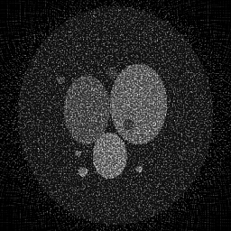
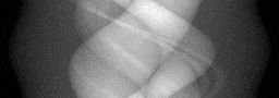
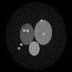
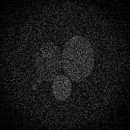
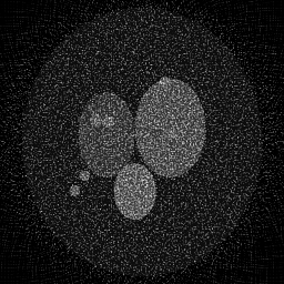
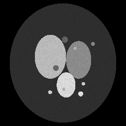
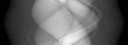
Experimental Setup — Signal Chain

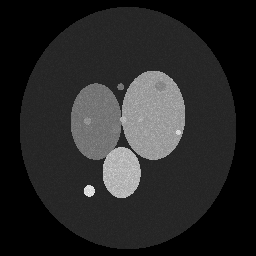
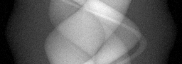
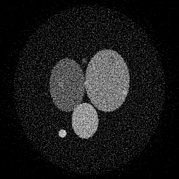
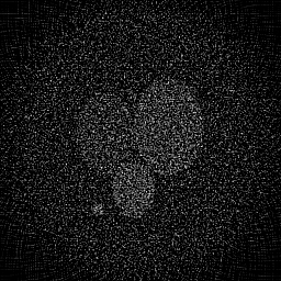
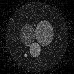
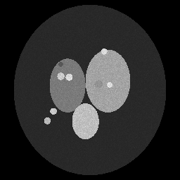
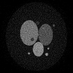
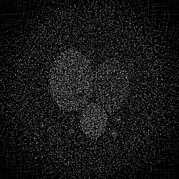
Reconstruction Gallery — 4 Scenes × 3 Scenarios
Method: CPU_baseline | Mismatch: nominal (nominal=True, perturbed=False)
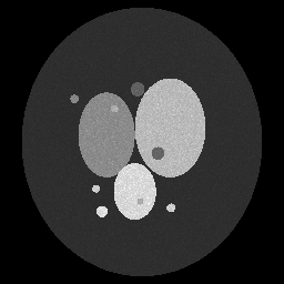
Ground Truth
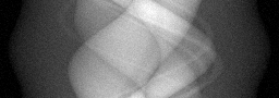
Measurement
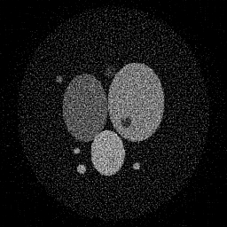
Reconstruction
Ground Truth

Measurement
Reconstruction
Ground Truth
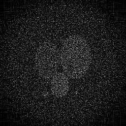
Measurement (perturbed)
Reconstruction


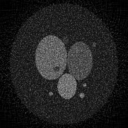
Mean PSNR Across All Scenes
Per-scene PSNR breakdown (4 scenes)
| Scene | I (PSNR) | I (SSIM) | II (PSNR) | II (SSIM) | III (PSNR) | III (SSIM) |
|---|---|---|---|---|---|---|
| scene_00 | 16.800662320808726 | 0.3125637672870015 | 12.496900330748657 | 0.043923207661581 | 15.939991231698041 | 0.12053931822727061 |
| scene_01 | 19.388438111108684 | 0.31563211467594515 | 13.982318112598847 | 0.048741115269095435 | 17.29916579028792 | 0.11442505385376642 |
| scene_02 | 18.671523249473616 | 0.31529580083957603 | 13.496104022434242 | 0.04800793047622927 | 16.7098923203481 | 0.12394712248370454 |
| scene_03 | 16.41438468401818 | 0.3200775078561238 | 12.526765088110148 | 0.043975715148042334 | 15.92079110351518 | 0.1230522724281324 |
| Mean | 17.8187520913523 | 0.31589229766466165 | 13.125521888472973 | 0.04616199213873701 | 16.467460111462312 | 0.12049094174821849 |
Experimental Setup
Key References
- Bercoff et al., 'Supersonic shear imaging: a new technique for soft tissue elasticity mapping', IEEE TUFFC 51, 396-409 (2004)
- Barr et al., 'Elastography assessment of liver fibrosis', Radiology 276, 845-861 (2015)
Canonical Datasets
- Clinical SWE liver fibrosis benchmark data
Spec DAG — Forward Model Pipeline
P(shear) → Σ_t → D(g, η₂)
Mismatch Parameters
| Symbol | Parameter | Description | Nominal | Perturbed |
|---|---|---|---|---|
| Δc_s | shear_speed | Shear speed error (m/s) | 0 | 0.3 |
| Δτ | push_duration | Push-pulse duration error (μs) | 0 | 10 |
| Δη | tissue_viscosity | Viscosity model error (%) | 0 | 15.0 |
Credits System
Spec Primitives Reference (11 primitives)
Free-space or medium propagation kernel (Fresnel, Rayleigh-Sommerfeld).
Spatial or spatio-temporal amplitude modulation (coded aperture, SLM pattern).
Geometric projection operator (Radon transform, fan-beam, cone-beam).
Sampling in the Fourier / k-space domain (MRI, ptychography).
Shift-invariant convolution with a point-spread function (PSF).
Summation along a physical dimension (spectral, temporal, angular).
Sensor readout with gain g and noise model η (Gaussian, Poisson, mixed).
Patterned illumination (block, Hadamard, random) applied to the scene.
Spectral dispersion element (prism, grating) with shift α and aperture a.
Sample or gantry rotation (CT, electron tomography).
Spectral filter or monochromator selecting a wavelength band.