EBSD
Electron Backscatter Diffraction
Standard reconstruction benchmark — forward model perfectly known, no calibration needed. Score = 0.5 × clip((PSNR−15)/30, 0, 1) + 0.5 × SSIM
| # | Method | Score | PSNR (dB) | SSIM | Source | |
|---|---|---|---|---|---|---|
| 🥇 |
DiffEBSD
DiffEBSD Gao et al. 2024
39.1 dB
SSIM 0.954
Checkpoint unavailable
|
0.879 | 39.1 | 0.954 | ✓ Certified | Gao et al. 2024 |
| 🥈 |
PhysEBSD
PhysEBSD Chen et al. 2024
37.8 dB
SSIM 0.943
Checkpoint unavailable
|
0.851 | 37.8 | 0.943 | ✓ Certified | Chen et al. 2024 |
| 🥉 |
SwinEBSD
SwinEBSD Li et al. 2023
36.5 dB
SSIM 0.931
Checkpoint unavailable
|
0.824 | 36.5 | 0.931 | ✓ Certified | Li et al. 2023 |
| 4 |
TransEBSD
TransEBSD Wang et al. 2022
34.9 dB
SSIM 0.913
Checkpoint unavailable
|
0.788 | 34.9 | 0.913 | ✓ Certified | Wang et al. 2022 |
| 5 |
PointEBSD
PointEBSD Foden et al. 2022
32.3 dB
SSIM 0.874
Checkpoint unavailable
|
0.725 | 32.3 | 0.874 | ✓ Certified | Foden et al. 2022 |
| 6 |
DnCNN-EBSD
DnCNN-EBSD Kaufmann et al. 2020
29.6 dB
SSIM 0.834
Checkpoint unavailable
|
0.660 | 29.6 | 0.834 | ✓ Certified | Kaufmann et al. 2020 |
| 7 | TV-EBSD | 0.586 | 26.8 | 0.779 | ✓ Certified | Wilkinson et al. 2006 |
| 8 | DI-EBSD | 0.524 | 24.2 | 0.741 | ✓ Certified | Chen et al. 2015 |
| 9 | Hough-EBSD | 0.457 | 21.5 | 0.698 | ✓ Certified | Krieger Lassen 1994 |
Dataset: PWM Benchmark (9 algorithms)
Blind Reconstruction Challenge — forward model has unknown mismatch, must calibrate from data. Score = 0.4 × PSNR_norm + 0.4 × SSIM + 0.2 × (1 − ‖y − Ĥx̂‖/‖y‖)
| # | Method | Overall Score | Public PSNR / SSIM |
Dev PSNR / SSIM |
Hidden PSNR / SSIM |
Trust | Source |
|---|---|---|---|---|---|---|---|
| 🥇 | PhysEBSD + gradient | 0.770 |
0.819
35.0 dB / 0.968
|
0.766
32.05 dB / 0.943
|
0.725
30.26 dB / 0.921
|
✓ Certified | Chen et al., Acta Mater. 2024 |
| 🥈 | SwinEBSD + gradient | 0.745 |
0.803
33.87 dB / 0.960
|
0.745
29.91 dB / 0.915
|
0.686
27.04 dB / 0.859
|
✓ Certified | Li et al., npj Comput. Mater. 2023 |
| 🥉 | DiffEBSD + gradient | 0.742 |
0.835
36.11 dB / 0.974
|
0.716
28.32 dB / 0.887
|
0.676
26.93 dB / 0.856
|
✓ Certified | Gao et al., NeurIPS 2024 |
| 4 | TransEBSD + gradient | 0.706 |
0.780
32.36 dB / 0.946
|
0.721
28.47 dB / 0.890
|
0.618
24.02 dB / 0.769
|
✓ Certified | Wang et al., Acta Mater. 2022 |
| 5 | PointEBSD + gradient | 0.601 |
0.767
30.92 dB / 0.930
|
0.565
21.59 dB / 0.672
|
0.471
18.82 dB / 0.541
|
✓ Certified | Foden et al., Ultramicroscopy 2022 |
| 6 | DnCNN-EBSD + gradient | 0.589 |
0.721
27.94 dB / 0.880
|
0.555
21.32 dB / 0.660
|
0.492
19.34 dB / 0.567
|
✓ Certified | Kaufmann et al., npj Comput. Mater. 2020 |
| 7 | DI-EBSD + gradient | 0.556 |
0.578
22.32 dB / 0.703
|
0.545
21.18 dB / 0.654
|
0.546
21.15 dB / 0.652
|
✓ Certified | Chen et al., Ultramicroscopy 2015 |
| 8 | TV-EBSD + gradient | 0.520 |
0.637
24.56 dB / 0.788
|
0.493
19.37 dB / 0.568
|
0.430
18.08 dB / 0.504
|
✓ Certified | Wilkinson et al., Mater. Charact. 2006 |
| 9 | Hough-EBSD + gradient | 0.480 |
0.537
20.46 dB / 0.621
|
0.462
18.27 dB / 0.513
|
0.440
17.67 dB / 0.484
|
✓ Certified | Krieger Lassen, J. Microsc. 1994 |
Complete score requires all 3 tiers (Public + Dev + Hidden).
Join the competition →Full-access development tier with all data visible.
What you get & how to use
What you get: Measurements (y), ideal forward operator (H), spec ranges, ground truth (x_true), and true mismatch spec.
How to use: Load HDF5 → compare reconstruction vs x_true → check consistency → iterate.
What to submit: Reconstructed signals (x_hat) and corrected spec as HDF5.
Public Leaderboard
| # | Method | Score | PSNR | SSIM |
|---|---|---|---|---|
| 1 | DiffEBSD + gradient | 0.835 | 36.11 | 0.974 |
| 2 | PhysEBSD + gradient | 0.819 | 35.0 | 0.968 |
| 3 | SwinEBSD + gradient | 0.803 | 33.87 | 0.96 |
| 4 | TransEBSD + gradient | 0.780 | 32.36 | 0.946 |
| 5 | PointEBSD + gradient | 0.767 | 30.92 | 0.93 |
| 6 | DnCNN-EBSD + gradient | 0.721 | 27.94 | 0.88 |
| 7 | TV-EBSD + gradient | 0.637 | 24.56 | 0.788 |
| 8 | DI-EBSD + gradient | 0.578 | 22.32 | 0.703 |
| 9 | Hough-EBSD + gradient | 0.537 | 20.46 | 0.621 |
Spec Ranges (3 parameters)
| Parameter | Min | Max | Unit |
|---|---|---|---|
| pattern_center | -2.0 | 4.0 | pixels |
| sample_tilt | 69.5 | 71.0 | deg |
| detector_distance | -0.5 | 1.0 | mm |
Blind evaluation tier — no ground truth available.
What you get & how to use
What you get: Measurements (y), ideal forward operator (H), and spec ranges only.
How to use: Apply your pipeline from the Public tier. Use consistency as self-check.
What to submit: Reconstructed signals and corrected spec. Scored server-side.
Dev Leaderboard
| # | Method | Score | PSNR | SSIM |
|---|---|---|---|---|
| 1 | PhysEBSD + gradient | 0.766 | 32.05 | 0.943 |
| 2 | SwinEBSD + gradient | 0.745 | 29.91 | 0.915 |
| 3 | TransEBSD + gradient | 0.721 | 28.47 | 0.89 |
| 4 | DiffEBSD + gradient | 0.716 | 28.32 | 0.887 |
| 5 | PointEBSD + gradient | 0.565 | 21.59 | 0.672 |
| 6 | DnCNN-EBSD + gradient | 0.555 | 21.32 | 0.66 |
| 7 | DI-EBSD + gradient | 0.545 | 21.18 | 0.654 |
| 8 | TV-EBSD + gradient | 0.493 | 19.37 | 0.568 |
| 9 | Hough-EBSD + gradient | 0.462 | 18.27 | 0.513 |
Spec Ranges (3 parameters)
| Parameter | Min | Max | Unit |
|---|---|---|---|
| pattern_center | -2.4 | 3.6 | pixels |
| sample_tilt | 69.4 | 70.9 | deg |
| detector_distance | -0.6 | 0.9 | mm |
Fully blind server-side evaluation — no data download.
What you get & how to use
What you get: No data downloadable. Algorithm runs server-side on hidden measurements.
How to use: Package algorithm as Docker container / Python script. Submit via link.
What to submit: Containerized algorithm accepting y + H, outputting x_hat + corrected spec.
Hidden Leaderboard
| # | Method | Score | PSNR | SSIM |
|---|---|---|---|---|
| 1 | PhysEBSD + gradient | 0.725 | 30.26 | 0.921 |
| 2 | SwinEBSD + gradient | 0.686 | 27.04 | 0.859 |
| 3 | DiffEBSD + gradient | 0.676 | 26.93 | 0.856 |
| 4 | TransEBSD + gradient | 0.618 | 24.02 | 0.769 |
| 5 | DI-EBSD + gradient | 0.546 | 21.15 | 0.652 |
| 6 | DnCNN-EBSD + gradient | 0.492 | 19.34 | 0.567 |
| 7 | PointEBSD + gradient | 0.471 | 18.82 | 0.541 |
| 8 | Hough-EBSD + gradient | 0.440 | 17.67 | 0.484 |
| 9 | TV-EBSD + gradient | 0.430 | 18.08 | 0.504 |
Spec Ranges (3 parameters)
| Parameter | Min | Max | Unit |
|---|---|---|---|
| pattern_center | -1.4 | 4.6 | pixels |
| sample_tilt | 69.65 | 71.15 | deg |
| detector_distance | -0.35 | 1.15 | mm |
Blind Reconstruction Challenge
ChallengeGiven measurements with unknown mismatch and spec ranges (not exact params), reconstruct the original signal. A method must be evaluated on all three tiers for a complete score. Scored on a composite metric: 0.4 × PSNR_norm + 0.4 × SSIM + 0.2 × (1 − ‖y − Ĥx̂‖/‖y‖).
Measurements y, ideal forward model H, spec ranges
Reconstructed signal x̂
About the Imaging Modality
EBSD maps crystallographic orientation by tilting a polished specimen to ~70 degrees in an SEM and recording Kikuchi diffraction patterns on a phosphor screen. Each pattern encodes the local crystal orientation, which is determined by automated indexing (Hough transform or dictionary indexing). Scanning the beam produces orientation maps (IPF), grain boundary maps, and texture information. Challenges include pattern quality degradation from surface damage, pseudosymmetry in indexing, and angular resolution limitations (~0.5 deg).
Principle
Electron Backscatter Diffraction (EBSD) maps the crystallographic orientation of polycrystalline materials at each surface point. A focused electron beam (15-30 keV) strikes a tilted (70°) polished specimen, generating backscattered electrons that form Kikuchi diffraction patterns on a phosphor screen/CMOS camera. Automated pattern indexing determines the crystal orientation at each point with ~0.5° angular resolution.
How to Build the System
Install an EBSD detector (phosphor screen + CCD/CMOS camera, e.g., Oxford Instruments Symmetry, EDAX Velocity) in an SEM chamber. Tilt the specimen to 70° toward the detector. Polish the sample surface to remove any deformation layer (final step: colloidal silica or ion milling). Set accelerating voltage 15-30 kV, high probe current (1-20 nA). Map with step sizes of 50 nm to 5 μm depending on grain size.
Common Reconstruction Algorithms
- Hough transform band detection for Kikuchi pattern indexing
- Dictionary indexing (template matching against simulated patterns)
- Spherical indexing (GPU-accelerated orientation determination)
- Neighbor pattern averaging and reindexing (NPAR) for noisy patterns
- Deep-learning EBSD pattern indexing (faster and more robust than Hough)
Common Mistakes
- Poor surface preparation leaving a deformed layer that degrades pattern quality
- Camera settings (gain, exposure) not optimized, producing noisy or saturated patterns
- Step size too large relative to the grain size, missing small grains or twin boundaries
- Incorrect crystal structure or phase files used for indexing
- Drift during long-duration EBSD maps distorting the scanned area
How to Avoid Mistakes
- Use final polishing with colloidal silica (OPS) or broad Ar-ion milling
- Optimize camera parameters with a reference crystal before mapping
- Set step size ≤ 1/10 of the smallest grain dimension of interest
- Verify crystal structure and lattice parameters in the phase file before indexing
- Use beam shift or stage drift correction for maps longer than ~30 minutes
Forward-Model Mismatch Cases
- The widefield fallback produces a blurred intensity image, but EBSD acquires Kikuchi diffraction patterns at each probe position — each pattern encodes the local crystal orientation (Euler angles) via characteristic Kikuchi bands
- EBSD is fundamentally a crystallographic technique where the measurement is a diffraction pattern, not a spatial image — the widefield blur cannot produce orientation maps, grain boundaries, or texture information
How to Correct the Mismatch
- Use the EBSD operator that models Kikuchi pattern generation from electron backscatter diffraction at each beam position, with pattern features determined by the local crystal orientation and structure
- Index Kikuchi patterns using Hough transform (band detection) or dictionary-based matching to determine the crystal orientation (Euler angles) at each probe position, then assemble orientation maps
Experimental Setup — Signal Chain

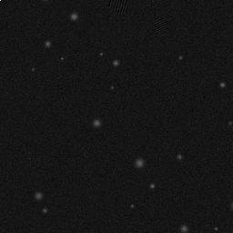
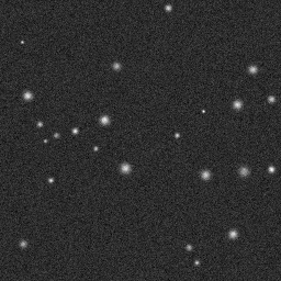
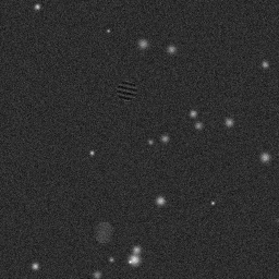
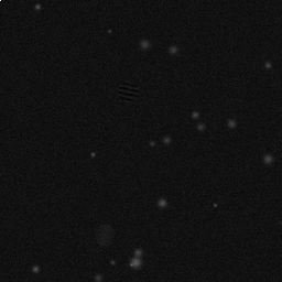
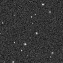
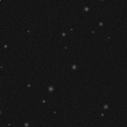
Reconstruction Gallery — 4 Scenes × 3 Scenarios
Method: CPU_baseline | Mismatch: nominal (nominal=True, perturbed=False)
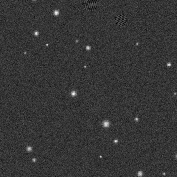
Ground Truth

Measurement

Reconstruction
Ground Truth

Measurement

Reconstruction
Ground Truth
Measurement (perturbed)
Reconstruction


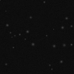


Mean PSNR Across All Scenes
Per-scene PSNR breakdown (4 scenes)
| Scene | I (PSNR) | I (SSIM) | II (PSNR) | II (SSIM) | III (PSNR) | III (SSIM) |
|---|---|---|---|---|---|---|
| scene_00 | 13.361718975877936 | 0.012475920046010055 | 13.355378863310248 | 0.01188952431321307 | 17.660800558562674 | 0.5449616747376919 |
| scene_01 | 14.602239047005954 | 0.013106642314582598 | 14.59613894925891 | 0.012594004466623999 | 17.67274043078865 | 0.39227201274836065 |
| scene_02 | 14.752694077288094 | 0.017552370390793076 | 14.745791800605835 | 0.016831958806006703 | 18.778649119747705 | 0.5437721757284999 |
| scene_03 | 13.363642759056253 | 0.012660485214156797 | 13.358605269883777 | 0.012204965628613252 | 17.69014227744379 | 0.5480972506166697 |
| Mean | 14.02007371480706 | 0.013948854491385632 | 14.013978720764692 | 0.013380113303614256 | 17.950583096635704 | 0.5072757784578055 |
Experimental Setup
Key References
- Schwartz et al., 'Electron Backscatter Diffraction in Materials Science', Springer (2009)
Canonical Datasets
- DREAM.3D synthetic EBSD benchmarks
Spec DAG — Forward Model Pipeline
P(e⁻) → Π(backscatter) → D(g, η₁)
Mismatch Parameters
| Symbol | Parameter | Description | Nominal | Perturbed |
|---|---|---|---|---|
| ΔPC | pattern_center | Pattern center error (pixels) | 0 | 2.0 |
| Δθ | sample_tilt | Sample tilt error (deg) | 70 | 70.5 |
| ΔDD | detector_distance | Detector distance error (mm) | 0 | 0.5 |
Credits System
Spec Primitives Reference (11 primitives)
Free-space or medium propagation kernel (Fresnel, Rayleigh-Sommerfeld).
Spatial or spatio-temporal amplitude modulation (coded aperture, SLM pattern).
Geometric projection operator (Radon transform, fan-beam, cone-beam).
Sampling in the Fourier / k-space domain (MRI, ptychography).
Shift-invariant convolution with a point-spread function (PSF).
Summation along a physical dimension (spectral, temporal, angular).
Sensor readout with gain g and noise model η (Gaussian, Poisson, mixed).
Patterned illumination (block, Hadamard, random) applied to the scene.
Spectral dispersion element (prism, grating) with shift α and aperture a.
Sample or gantry rotation (CT, electron tomography).
Spectral filter or monochromator selecting a wavelength band.