DOT
Diffuse Optical Tomography
Standard reconstruction benchmark — forward model perfectly known, no calibration needed. Score = 0.5 × clip((PSNR−15)/30, 0, 1) + 0.5 × SSIM
| # | Method | Score | PSNR (dB) | SSIM | Source | |
|---|---|---|---|---|---|---|
| 🥇 |
DiffusionDOT
DiffusionDOT Gao et al. 2024
39.0 dB
SSIM 0.954
Checkpoint unavailable
|
0.877 | 39.0 | 0.954 | ✓ Certified | Gao et al. 2024 |
| 🥈 |
PhysDOT
PhysDOT Chen et al. 2024
37.5 dB
SSIM 0.942
Checkpoint unavailable
|
0.846 | 37.5 | 0.942 | ✓ Certified | Chen et al. 2024 |
| 🥉 |
SwinDOT
SwinDOT Wang et al. 2023
36.1 dB
SSIM 0.930
Checkpoint unavailable
|
0.817 | 36.1 | 0.930 | ✓ Certified | Wang et al. 2023 |
| 4 |
TransDOT
TransDOT Li et al. 2022
34.2 dB
SSIM 0.910
Checkpoint unavailable
|
0.775 | 34.2 | 0.910 | ✓ Certified | Li et al. 2022 |
| 5 |
DOT-Net
DOT-Net Guo et al. 2021
31.4 dB
SSIM 0.868
Checkpoint unavailable
|
0.707 | 31.4 | 0.868 | ✓ Certified | Guo et al. 2021 |
| 6 |
DnCNN-DOT
DnCNN-DOT Yoo et al. 2019
28.7 dB
SSIM 0.825
Checkpoint unavailable
|
0.641 | 28.7 | 0.825 | ✓ Certified | Yoo et al. 2019 |
| 7 | FEM-DOT | 0.567 | 25.9 | 0.771 | ✓ Certified | Schweiger et al. 2005 |
| 8 | TV-DOT | 0.506 | 23.5 | 0.729 | ✓ Certified | Borsic et al., IEEE TMI 2010 |
| 9 | Born-Approx | 0.437 | 20.8 | 0.681 | ✓ Certified | Arridge, Inverse Probl. 1999 |
Dataset: PWM Benchmark (9 algorithms)
Blind Reconstruction Challenge — forward model has unknown mismatch, must calibrate from data. Score = 0.4 × PSNR_norm + 0.4 × SSIM + 0.2 × (1 − ‖y − Ĥx̂‖/‖y‖)
| # | Method | Overall Score | Public PSNR / SSIM |
Dev PSNR / SSIM |
Hidden PSNR / SSIM |
Trust | Source |
|---|---|---|---|---|---|---|---|
| 🥇 | DiffusionDOT + gradient | 0.787 |
0.835
36.94 dB / 0.978
|
0.788
33.47 dB / 0.957
|
0.739
29.98 dB / 0.917
|
✓ Certified | Gao et al., NeurIPS 2024 |
| 🥈 | PhysDOT + gradient | 0.752 |
0.815
35.18 dB / 0.969
|
0.739
29.65 dB / 0.911
|
0.701
28.25 dB / 0.886
|
✓ Certified | Chen et al., Opt. Express 2024 |
| 🥉 | SwinDOT + gradient | 0.738 |
0.821
34.82 dB / 0.967
|
0.727
29.87 dB / 0.915
|
0.666
26.85 dB / 0.854
|
✓ Certified | Wang et al., Biomed. Opt. Express 2023 |
| 4 | TransDOT + gradient | 0.735 |
0.775
32.28 dB / 0.946
|
0.733
29.49 dB / 0.909
|
0.697
27.8 dB / 0.877
|
✓ Certified | Li et al., IEEE TMI 2022 |
| 5 | FEM-DOT + gradient | 0.599 |
0.607
23.11 dB / 0.735
|
0.595
23.42 dB / 0.747
|
0.595
23.25 dB / 0.741
|
✓ Certified | Schweiger et al., J. Biomed. Opt. 2005 |
| 6 | DOT-Net + gradient | 0.560 |
0.730
29.33 dB / 0.906
|
0.517
20.68 dB / 0.631
|
0.433
17.55 dB / 0.478
|
✓ Certified | Guo et al., Biomed. Opt. Express 2021 |
| 7 | DnCNN-DOT + gradient | 0.532 |
0.707
27.39 dB / 0.867
|
0.498
19.76 dB / 0.587
|
0.390
15.97 dB / 0.400
|
✓ Certified | Yoo et al., Sci. Rep. 2019 |
| 8 | Born-Approx + gradient | 0.440 |
0.502
19.08 dB / 0.554
|
0.423
17.35 dB / 0.468
|
0.396
16.38 dB / 0.420
|
✓ Certified | Arridge, Inverse Probl. 1999 |
| 9 | TV-DOT + gradient | 0.389 |
0.559
21.59 dB / 0.672
|
0.358
14.99 dB / 0.354
|
0.251
11.42 dB / 0.211
|
✓ Certified | Borsic et al., IEEE TMI 2010 |
Complete score requires all 3 tiers (Public + Dev + Hidden).
Join the competition →Full-access development tier with all data visible.
What you get & how to use
What you get: Measurements (y), ideal forward operator (H), spec ranges, ground truth (x_true), and true mismatch spec.
How to use: Load HDF5 → compare reconstruction vs x_true → check consistency → iterate.
What to submit: Reconstructed signals (x_hat) and corrected spec as HDF5.
Public Leaderboard
| # | Method | Score | PSNR | SSIM |
|---|---|---|---|---|
| 1 | DiffusionDOT + gradient | 0.835 | 36.94 | 0.978 |
| 2 | SwinDOT + gradient | 0.821 | 34.82 | 0.967 |
| 3 | PhysDOT + gradient | 0.815 | 35.18 | 0.969 |
| 4 | TransDOT + gradient | 0.775 | 32.28 | 0.946 |
| 5 | DOT-Net + gradient | 0.730 | 29.33 | 0.906 |
| 6 | DnCNN-DOT + gradient | 0.707 | 27.39 | 0.867 |
| 7 | FEM-DOT + gradient | 0.607 | 23.11 | 0.735 |
| 8 | TV-DOT + gradient | 0.559 | 21.59 | 0.672 |
| 9 | Born-Approx + gradient | 0.502 | 19.08 | 0.554 |
Spec Ranges (3 parameters)
| Parameter | Min | Max | Unit |
|---|---|---|---|
| mu_a | -10.0 | 20.0 | % |
| mu_s | -8.0 | 16.0 | % |
| source_pos | -1.0 | 2.0 | mm |
Blind evaluation tier — no ground truth available.
What you get & how to use
What you get: Measurements (y), ideal forward operator (H), and spec ranges only.
How to use: Apply your pipeline from the Public tier. Use consistency as self-check.
What to submit: Reconstructed signals and corrected spec. Scored server-side.
Dev Leaderboard
| # | Method | Score | PSNR | SSIM |
|---|---|---|---|---|
| 1 | DiffusionDOT + gradient | 0.788 | 33.47 | 0.957 |
| 2 | PhysDOT + gradient | 0.739 | 29.65 | 0.911 |
| 3 | TransDOT + gradient | 0.733 | 29.49 | 0.909 |
| 4 | SwinDOT + gradient | 0.727 | 29.87 | 0.915 |
| 5 | FEM-DOT + gradient | 0.595 | 23.42 | 0.747 |
| 6 | DOT-Net + gradient | 0.517 | 20.68 | 0.631 |
| 7 | DnCNN-DOT + gradient | 0.498 | 19.76 | 0.587 |
| 8 | Born-Approx + gradient | 0.423 | 17.35 | 0.468 |
| 9 | TV-DOT + gradient | 0.358 | 14.99 | 0.354 |
Spec Ranges (3 parameters)
| Parameter | Min | Max | Unit |
|---|---|---|---|
| mu_a | -12.0 | 18.0 | % |
| mu_s | -9.6 | 14.4 | % |
| source_pos | -1.2 | 1.8 | mm |
Fully blind server-side evaluation — no data download.
What you get & how to use
What you get: No data downloadable. Algorithm runs server-side on hidden measurements.
How to use: Package algorithm as Docker container / Python script. Submit via link.
What to submit: Containerized algorithm accepting y + H, outputting x_hat + corrected spec.
Hidden Leaderboard
| # | Method | Score | PSNR | SSIM |
|---|---|---|---|---|
| 1 | DiffusionDOT + gradient | 0.739 | 29.98 | 0.917 |
| 2 | PhysDOT + gradient | 0.701 | 28.25 | 0.886 |
| 3 | TransDOT + gradient | 0.697 | 27.8 | 0.877 |
| 4 | SwinDOT + gradient | 0.666 | 26.85 | 0.854 |
| 5 | FEM-DOT + gradient | 0.595 | 23.25 | 0.741 |
| 6 | DOT-Net + gradient | 0.433 | 17.55 | 0.478 |
| 7 | Born-Approx + gradient | 0.396 | 16.38 | 0.42 |
| 8 | DnCNN-DOT + gradient | 0.390 | 15.97 | 0.4 |
| 9 | TV-DOT + gradient | 0.251 | 11.42 | 0.211 |
Spec Ranges (3 parameters)
| Parameter | Min | Max | Unit |
|---|---|---|---|
| mu_a | -7.0 | 23.0 | % |
| mu_s | -5.6 | 18.4 | % |
| source_pos | -0.7 | 2.3 | mm |
Blind Reconstruction Challenge
ChallengeGiven measurements with unknown mismatch and spec ranges (not exact params), reconstruct the original signal. A method must be evaluated on all three tiers for a complete score. Scored on a composite metric: 0.4 × PSNR_norm + 0.4 × SSIM + 0.2 × (1 − ‖y − Ĥx̂‖/‖y‖).
Measurements y, ideal forward model H, spec ranges
Reconstructed signal x̂
About the Imaging Modality
Diffuse optical tomography (DOT) reconstructs 3D maps of tissue optical properties (absorption mu_a and reduced scattering mu_s') by measuring near-infrared light transport through highly scattering tissue. Multiple source-detector pairs on the tissue surface sample the diffuse photon field. The forward model is the diffusion equation: light propagation is modelled as a diffusive process with the photon fluence depending on the spatial distribution of mu_a and mu_s'. Reconstruction linearizes around a homogeneous background (Born/Rytov approximation) or uses nonlinear iterative methods. Applications include breast imaging and functional brain imaging (fNIRS-DOT).
Principle
Diffuse Optical Tomography reconstructs 3-D maps of tissue optical properties (absorption μₐ and reduced scattering μ'ₛ) from measurements of multiply scattered near-infrared light transmitted through tissue. Multiple source-detector pairs on the tissue surface provide overlapping sensitivity profiles. The diffusion equation models light propagation in the multiple-scattering regime.
How to Build the System
Place fiber-coupled NIR sources (670-850 nm laser diodes, CW or frequency-domain modulated at 100-300 MHz, or time-domain pulsed) and detector fibers (avalanche photodiodes or PMTs) on the tissue surface in an array. A multiplexer switches between source positions. For breast DOT, 32-128 optode positions on a cup or ring geometry. Calibrate with known optical phantoms (Intralipid + ink solutions).
Common Reconstruction Algorithms
- Normalized Born approximation (linearized diffuse optical tomography)
- Nonlinear Newton-type iterative reconstruction (Gauss-Newton, Levenberg-Marquardt)
- Finite-element method (FEM) based forward solver + Tikhonov regularization
- TOAST++ (Time-resolved Optical Absorption and Scattering Tomography)
- Deep-learning DOT (learned regularization, direct inversion networks)
Common Mistakes
- Poor optode-tissue coupling due to hair, uneven surfaces, or insufficient pressure
- Inadequate source-detector pair coverage causing reconstruction blind spots
- Cross-talk between source channels if multiplexing is not properly timed
- Using the diffusion approximation too close to sources or in low-scattering regions
- Ignoring tissue heterogeneity in the background optical property estimate
How to Avoid Mistakes
- Use spring-loaded optodes with coupling checks; shave hair in the measurement area
- Design source-detector geometry with overlapping sensitivity to cover the volume of interest
- Ensure clean channel switching with adequate settling time between multiplexed measurements
- Use higher-order transport models (radiative transfer) near sources if needed
- Initialize reconstruction with patient-specific anatomical prior (from MRI or CT)
Forward-Model Mismatch Cases
- The widefield fallback produces a 2D (64,64) image, but Diffuse Optical Tomography acquires boundary measurements (source-detector pairs) — output shape (64,) is a 1D vector of photon counts at detector positions
- DOT measurement physics involves diffuse light propagation through scattering tissue (modeled by the diffusion equation), which is fundamentally different from surface-level Gaussian blur — the fallback cannot model subsurface absorption and scattering
How to Correct the Mismatch
- Use the DOT operator that models photon transport via the diffusion equation: Jacobian maps from interior optical properties (absorption, scattering) to boundary measurements at each source-detector pair
- Reconstruct interior absorption/scattering maps using Tikhonov-regularized inversion or iterative methods (conjugate gradient) with the correct diffusion-equation-based forward model
Experimental Setup — Signal Chain

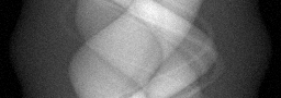
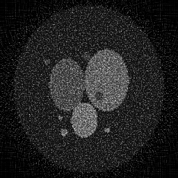
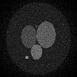
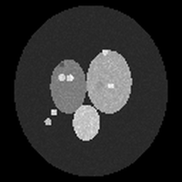
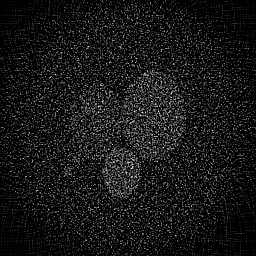
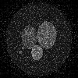
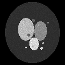
Reconstruction Gallery — 4 Scenes × 3 Scenarios
Method: CPU_baseline | Mismatch: nominal (nominal=True, perturbed=False)

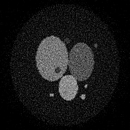
Ground Truth
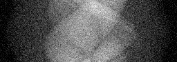
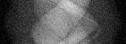
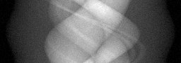
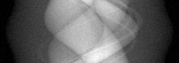
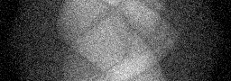
Measurement
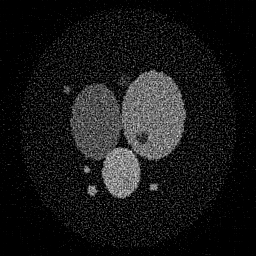
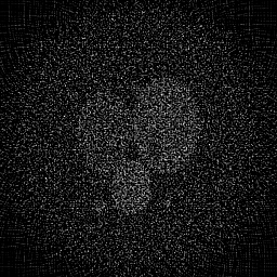
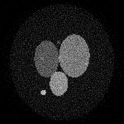
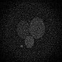
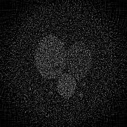
Reconstruction
Ground Truth
Measurement
Reconstruction
Ground Truth
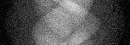
Measurement (perturbed)
Reconstruction


Mean PSNR Across All Scenes
Per-scene PSNR breakdown (4 scenes)
| Scene | I (PSNR) | I (SSIM) | II (PSNR) | II (SSIM) | III (PSNR) | III (SSIM) |
|---|---|---|---|---|---|---|
| scene_00 | 16.584200964385797 | 0.3250905580130585 | 12.506523882319042 | 0.044716474341606735 | 15.931719256055723 | 0.12142227244746187 |
| scene_01 | 18.884299556167566 | 0.3252411352628261 | 13.742128073130111 | 0.048029248758291385 | 17.02391116326154 | 0.11622117666622035 |
| scene_02 | 18.301830801494646 | 0.32976160086547746 | 13.36792873190369 | 0.04964364838717723 | 16.550610792224443 | 0.1259030967011571 |
| scene_03 | 16.67775192548055 | 0.3247822274360334 | 12.53195005733068 | 0.044966709218701925 | 15.850507045662987 | 0.12621817875162467 |
| Mean | 17.61202081188214 | 0.3262188803943489 | 13.037132686170882 | 0.046839020176444326 | 16.33918706430117 | 0.122441181141616 |
Experimental Setup
Key References
- Arridge, 'Optical tomography in medical imaging', Inverse Problems 15, R41-R93 (1999)
- Boas et al., 'Imaging the body with diffuse optical tomography', IEEE Signal Processing Magazine 18, 57-75 (2001)
Canonical Datasets
- UCL DOT phantom datasets
- BU fNIRS-DOT brain imaging benchmarks
Spec DAG — Forward Model Pipeline
P(diffuse) → Σ → D(g, η₃)
Mismatch Parameters
| Symbol | Parameter | Description | Nominal | Perturbed |
|---|---|---|---|---|
| Δμ_a | mu_a | Absorption coefficient error (%) | 0 | 10.0 |
| Δμ_s' | mu_s | Reduced scattering error (%) | 0 | 8.0 |
| Δr_s | source_pos | Source position error (mm) | 0 | 1.0 |
Credits System
Spec Primitives Reference (11 primitives)
Free-space or medium propagation kernel (Fresnel, Rayleigh-Sommerfeld).
Spatial or spatio-temporal amplitude modulation (coded aperture, SLM pattern).
Geometric projection operator (Radon transform, fan-beam, cone-beam).
Sampling in the Fourier / k-space domain (MRI, ptychography).
Shift-invariant convolution with a point-spread function (PSF).
Summation along a physical dimension (spectral, temporal, angular).
Sensor readout with gain g and noise model η (Gaussian, Poisson, mixed).
Patterned illumination (block, Hadamard, random) applied to the scene.
Spectral dispersion element (prism, grating) with shift α and aperture a.
Sample or gantry rotation (CT, electron tomography).
Spectral filter or monochromator selecting a wavelength band.