Diffusion MRI
Diffusion MRI (DTI)
Standard reconstruction benchmark — forward model perfectly known, no calibration needed. Score = 0.5 × clip((PSNR−15)/30, 0, 1) + 0.5 × SSIM
| # | Method | Score | PSNR (dB) | SSIM | Source | |
|---|---|---|---|---|---|---|
| 🥇 |
DiffusionDTI
DiffusionDTI Gao et al., NeurIPS 2024
39.1 dB
SSIM 0.952
Checkpoint unavailable
|
0.878 | 39.1 | 0.952 | ✓ Certified | Gao et al., NeurIPS 2024 |
| 🥈 |
PhysDiffMRI
PhysDiffMRI Chen et al., MRM 2024
37.5 dB
SSIM 0.941
Checkpoint unavailable
|
0.845 | 37.5 | 0.941 | ✓ Certified | Chen et al., MRM 2024 |
| 🥉 |
SwinDTI
SwinDTI Wang et al., MICCAI 2023
36.2 dB
SSIM 0.931
Checkpoint unavailable
|
0.819 | 36.2 | 0.931 | ✓ Certified | Wang et al., MICCAI 2023 |
| 4 |
DTIFormer
DTIFormer Liu et al., MICCAI 2022
34.8 dB
SSIM 0.912
Checkpoint unavailable
|
0.786 | 34.8 | 0.912 | ✓ Certified | Liu et al., MICCAI 2022 |
| 5 |
DWIML-Net
DWIML-Net Qin et al., IEEE TMI 2019
32.1 dB
SSIM 0.871
Checkpoint unavailable
|
0.721 | 32.1 | 0.871 | ✓ Certified | Qin et al., IEEE TMI 2019 |
| 6 |
DnCNN-DTI
DnCNN-DTI Golkov et al., IEEE TMI 2016
29.3 dB
SSIM 0.831
Checkpoint unavailable
|
0.654 | 29.3 | 0.831 | ✓ Certified | Golkov et al., IEEE TMI 2016 |
| 7 | CHARMED | 0.588 | 26.8 | 0.782 | ✓ Certified | Assaf & Basser, NeuroImage 2005 |
| 8 | SHORE | 0.532 | 24.6 | 0.745 | ✓ Certified | Merlet & Deriche, MRM 2013 |
| 9 | DTI-FIT | 0.478 | 22.4 | 0.710 | ✓ Certified | Behrens et al., MRM 2003 |
Dataset: PWM Benchmark (9 algorithms)
Blind Reconstruction Challenge — forward model has unknown mismatch, must calibrate from data. Score = 0.4 × PSNR_norm + 0.4 × SSIM + 0.2 × (1 − ‖y − Ĥx̂‖/‖y‖)
| # | Method | Overall Score | Public PSNR / SSIM |
Dev PSNR / SSIM |
Hidden PSNR / SSIM |
Trust | Source |
|---|---|---|---|---|---|---|---|
| 🥇 | DiffusionDTI + gradient | 0.777 |
0.858
37.87 dB / 0.982
|
0.750
31.4 dB / 0.936
|
0.724
29.08 dB / 0.902
|
✓ Certified | Gao et al., NeurIPS 2024 |
| 🥈 | PhysDiffMRI + gradient | 0.752 |
0.818
35.69 dB / 0.972
|
0.743
30.15 dB / 0.919
|
0.696
27.77 dB / 0.876
|
✓ Certified | Chen et al., MRM 2024 |
| 🥉 | SwinDTI + gradient | 0.725 |
0.802
34.43 dB / 0.964
|
0.724
28.85 dB / 0.898
|
0.650
26.34 dB / 0.841
|
✓ Certified | Wang et al., MICCAI 2023 |
| 4 | DTIFormer + gradient | 0.723 |
0.783
32.87 dB / 0.951
|
0.713
28.48 dB / 0.891
|
0.672
27.23 dB / 0.864
|
✓ Certified | Liu et al., MICCAI 2022 |
| 5 | DWIML-Net + gradient | 0.662 |
0.764
30.61 dB / 0.926
|
0.635
25.0 dB / 0.802
|
0.588
23.08 dB / 0.734
|
✓ Certified | Qin et al., IEEE TMI 2019 |
| 6 | DnCNN-DTI + gradient | 0.589 |
0.693
27.18 dB / 0.862
|
0.559
21.67 dB / 0.676
|
0.516
20.08 dB / 0.603
|
✓ Certified | Golkov et al., IEEE TMI 2016 |
| 7 | SHORE + gradient | 0.576 |
0.614
23.16 dB / 0.737
|
0.577
22.65 dB / 0.717
|
0.536
21.5 dB / 0.668
|
✓ Certified | Merlet & Deriche, MRM 2013 |
| 8 | CHARMED + gradient | 0.500 |
0.668
25.48 dB / 0.817
|
0.435
17.84 dB / 0.492
|
0.397
16.48 dB / 0.425
|
✓ Certified | Assaf & Basser, NeuroImage 2005 |
| 9 | DTI-FIT + gradient | 0.471 |
0.512
19.76 dB / 0.587
|
0.467
18.45 dB / 0.522
|
0.434
17.99 dB / 0.500
|
✓ Certified | Behrens et al., MRM 2003 |
Complete score requires all 3 tiers (Public + Dev + Hidden).
Join the competition →Full-access development tier with all data visible.
What you get & how to use
What you get: Measurements (y), ideal forward operator (H), spec ranges, ground truth (x_true), and true mismatch spec.
How to use: Load HDF5 → compare reconstruction vs x_true → check consistency → iterate.
What to submit: Reconstructed signals (x_hat) and corrected spec as HDF5.
Public Leaderboard
| # | Method | Score | PSNR | SSIM |
|---|---|---|---|---|
| 1 | DiffusionDTI + gradient | 0.858 | 37.87 | 0.982 |
| 2 | PhysDiffMRI + gradient | 0.818 | 35.69 | 0.972 |
| 3 | SwinDTI + gradient | 0.802 | 34.43 | 0.964 |
| 4 | DTIFormer + gradient | 0.783 | 32.87 | 0.951 |
| 5 | DWIML-Net + gradient | 0.764 | 30.61 | 0.926 |
| 6 | DnCNN-DTI + gradient | 0.693 | 27.18 | 0.862 |
| 7 | CHARMED + gradient | 0.668 | 25.48 | 0.817 |
| 8 | SHORE + gradient | 0.614 | 23.16 | 0.737 |
| 9 | DTI-FIT + gradient | 0.512 | 19.76 | 0.587 |
Spec Ranges (4 parameters)
| Parameter | Min | Max | Unit |
|---|---|---|---|
| b_value_error | -3.0 | 6.0 | % |
| eddy_current | -0.5 | 1.0 | voxels |
| gradient_direction | -1.0 | 2.0 | deg |
| susceptibility | -1.0 | 2.0 | voxels |
Blind evaluation tier — no ground truth available.
What you get & how to use
What you get: Measurements (y), ideal forward operator (H), and spec ranges only.
How to use: Apply your pipeline from the Public tier. Use consistency as self-check.
What to submit: Reconstructed signals and corrected spec. Scored server-side.
Dev Leaderboard
| # | Method | Score | PSNR | SSIM |
|---|---|---|---|---|
| 1 | DiffusionDTI + gradient | 0.750 | 31.4 | 0.936 |
| 2 | PhysDiffMRI + gradient | 0.743 | 30.15 | 0.919 |
| 3 | SwinDTI + gradient | 0.724 | 28.85 | 0.898 |
| 4 | DTIFormer + gradient | 0.713 | 28.48 | 0.891 |
| 5 | DWIML-Net + gradient | 0.635 | 25.0 | 0.802 |
| 6 | SHORE + gradient | 0.577 | 22.65 | 0.717 |
| 7 | DnCNN-DTI + gradient | 0.559 | 21.67 | 0.676 |
| 8 | DTI-FIT + gradient | 0.467 | 18.45 | 0.522 |
| 9 | CHARMED + gradient | 0.435 | 17.84 | 0.492 |
Spec Ranges (4 parameters)
| Parameter | Min | Max | Unit |
|---|---|---|---|
| b_value_error | -3.6 | 5.4 | % |
| eddy_current | -0.6 | 0.9 | voxels |
| gradient_direction | -1.2 | 1.8 | deg |
| susceptibility | -1.2 | 1.8 | voxels |
Fully blind server-side evaluation — no data download.
What you get & how to use
What you get: No data downloadable. Algorithm runs server-side on hidden measurements.
How to use: Package algorithm as Docker container / Python script. Submit via link.
What to submit: Containerized algorithm accepting y + H, outputting x_hat + corrected spec.
Hidden Leaderboard
| # | Method | Score | PSNR | SSIM |
|---|---|---|---|---|
| 1 | DiffusionDTI + gradient | 0.724 | 29.08 | 0.902 |
| 2 | PhysDiffMRI + gradient | 0.696 | 27.77 | 0.876 |
| 3 | DTIFormer + gradient | 0.672 | 27.23 | 0.864 |
| 4 | SwinDTI + gradient | 0.650 | 26.34 | 0.841 |
| 5 | DWIML-Net + gradient | 0.588 | 23.08 | 0.734 |
| 6 | SHORE + gradient | 0.536 | 21.5 | 0.668 |
| 7 | DnCNN-DTI + gradient | 0.516 | 20.08 | 0.603 |
| 8 | DTI-FIT + gradient | 0.434 | 17.99 | 0.5 |
| 9 | CHARMED + gradient | 0.397 | 16.48 | 0.425 |
Spec Ranges (4 parameters)
| Parameter | Min | Max | Unit |
|---|---|---|---|
| b_value_error | -2.1 | 6.9 | % |
| eddy_current | -0.35 | 1.15 | voxels |
| gradient_direction | -0.7 | 2.3 | deg |
| susceptibility | -0.7 | 2.3 | voxels |
Blind Reconstruction Challenge
ChallengeGiven measurements with unknown mismatch and spec ranges (not exact params), reconstruct the original signal. A method must be evaluated on all three tiers for a complete score. Scored on a composite metric: 0.4 × PSNR_norm + 0.4 × SSIM + 0.2 × (1 − ‖y − Ĥx̂‖/‖y‖).
Measurements y, ideal forward model H, spec ranges
Reconstructed signal x̂
About the Imaging Modality
Diffusion MRI measures the random Brownian motion of water molecules in tissue by applying magnetic field gradient pulses that encode microscopic displacement. The signal attenuation follows S = S_0 * exp(-b * D_eff) where b is the diffusion weighting factor and D_eff is the effective diffusion coefficient along the gradient direction. Acquiring measurements in multiple gradient directions enables estimation of the diffusion tensor (DTI) and derived scalar maps (FA, MD, AD, RD). Advanced models (NODDI, CSD) resolve intra-voxel fiber crossings. Primary degradations include EPI distortion, eddy currents, and motion sensitivity.
Principle
Diffusion MRI sensitizes the MR signal to the Brownian motion of water molecules by applying strong magnetic field gradient pulses (Stejskal-Tanner scheme). In fibrous tissue (e.g., white matter), water diffuses preferentially along fibers, creating directional diffusion anisotropy. Diffusion Tensor Imaging (DTI) models this as a 3×3 tensor; higher-order models (HARDI, CSD) resolve crossing fibers.
How to Build the System
Acquire on a 3T scanner with high-performance gradients (80 mT/m, 200 T/m/s). Use spin-echo EPI with multiple b-values (e.g., b=0, 1000, 2000 s/mm²) and 30-300 diffusion directions uniformly distributed on the sphere. Include reverse-phase-encode b=0 images for EPI distortion correction. Multi-band (SMS) acceleration reduces scan time. Typical parameters: 2 mm isotropic, TE 60-90 ms, TR 3-5 s.
Common Reconstruction Algorithms
- DTI tensor fitting (least-squares or weighted least-squares)
- CSD (Constrained Spherical Deconvolution) for fiber orientation distribution
- NODDI (Neurite Orientation Dispersion and Density Imaging)
- Probabilistic tractography (FSL probtrackx, MRtrix3 iFOD2)
- Deep-learning tract segmentation (TractSeg, DeepBundle)
Common Mistakes
- Eddy current and EPI geometric distortions not corrected, causing tract errors
- Insufficient number of diffusion directions for the chosen model complexity
- Using DTI in regions with crossing fibers, producing incorrect FA and tract directions
- Susceptibility-induced signal dropout near air-tissue interfaces (sinuses, temporal lobes)
- Head motion between diffusion volumes causing inter-volume misalignment
How to Avoid Mistakes
- Apply FSL eddy or equivalent for eddy current, motion, and susceptibility correction
- Use ≥30 directions for DTI, ≥60 for CSD, and ≥90 for multi-shell models
- Use multi-fiber models (CSD, NODDI) in regions known to have crossing fibers
- Use reduced FOV or multi-shot EPI near susceptibility-prone regions
- Include interspersed b=0 volumes for robust motion and drift correction
Forward-Model Mismatch Cases
- The widefield fallback produces a blurred spatial image, but diffusion MRI applies magnetic field gradients to encode Brownian water motion — the Stejskal-Tanner signal attenuation S = S_0*exp(-b*D) is not modeled
- Diffusion MRI acquires multiple volumes at different b-values and gradient directions to measure the diffusion tensor at each voxel — the widefield single-image model cannot encode directional water diffusivity or fiber orientation
How to Correct the Mismatch
- Use the diffusion MRI operator that applies Stejskal-Tanner encoding: y_i = FFT(x * exp(-b_i * g_i^T * D * g_i)) for each gradient direction g_i and b-value b_i
- Reconstruct diffusion tensors (DTI) or fiber orientation distributions (CSD, NODDI) from the multi-direction, multi-b-value measurements using the correct diffusion-weighted forward model
Experimental Setup — Signal Chain

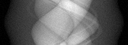
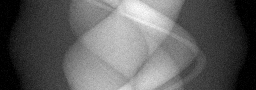
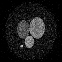
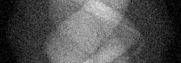
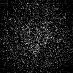
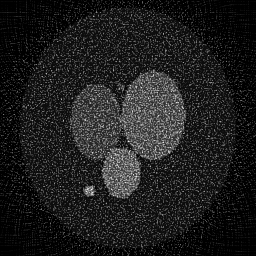
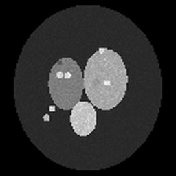
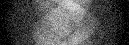
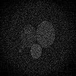
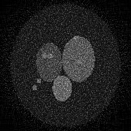
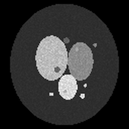
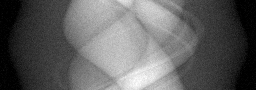
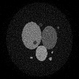
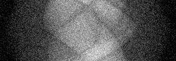
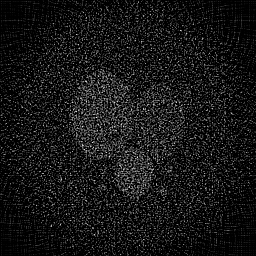
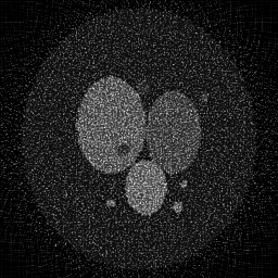
Reconstruction Gallery — 4 Scenes × 3 Scenarios
Method: CPU_baseline | Mismatch: nominal (nominal=True, perturbed=False)

Ground Truth
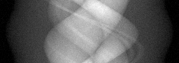
Measurement

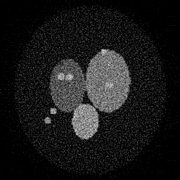
Reconstruction
Ground Truth
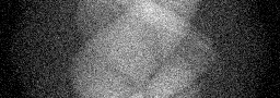
Measurement
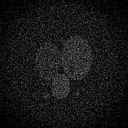
Reconstruction
Ground Truth
Measurement (perturbed)
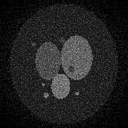
Reconstruction

Mean PSNR Across All Scenes
Per-scene PSNR breakdown (4 scenes)
| Scene | I (PSNR) | I (SSIM) | II (PSNR) | II (SSIM) | III (PSNR) | III (SSIM) |
|---|---|---|---|---|---|---|
| scene_00 | 16.584200964385797 | 0.3250905580130585 | 12.506523882319042 | 0.044716474341606735 | 15.931719256055723 | 0.12142227244746187 |
| scene_01 | 18.884299556167566 | 0.3252411352628261 | 13.742128073130111 | 0.048029248758291385 | 17.02391116326154 | 0.11622117666622035 |
| scene_02 | 18.301830801494646 | 0.32976160086547746 | 13.36792873190369 | 0.04964364838717723 | 16.550610792224443 | 0.1259030967011571 |
| scene_03 | 16.67775192548055 | 0.3247822274360334 | 12.53195005733068 | 0.044966709218701925 | 15.850507045662987 | 0.12621817875162467 |
| Mean | 17.61202081188214 | 0.3262188803943489 | 13.037132686170882 | 0.046839020176444326 | 16.33918706430117 | 0.122441181141616 |
Experimental Setup
Key References
- Basser et al., 'MR diffusion tensor spectroscopy and imaging', Biophysical Journal 66, 259-267 (1994)
- Sotiropoulos et al., 'Advances in diffusion MRI acquisition and processing in the HCP', NeuroImage 80, 125-143 (2013)
Canonical Datasets
- Human Connectome Project (HCP) diffusion data
- UK Biobank diffusion imaging
Spec DAG — Forward Model Pipeline
F(EPI) → D(g, η₁)
Mismatch Parameters
| Symbol | Parameter | Description | Nominal | Perturbed |
|---|---|---|---|---|
| Δb | b_value_error | b-value calibration error (%) | 0 | 3.0 |
| ε | eddy_current | Eddy-current distortion (voxels) | 0 | 0.5 |
| Δĝ | gradient_direction | Gradient direction error (deg) | 0 | 1.0 |
| Δχ | susceptibility | Susceptibility distortion (voxels) | 0 | 1.0 |
Credits System
Spec Primitives Reference (11 primitives)
Free-space or medium propagation kernel (Fresnel, Rayleigh-Sommerfeld).
Spatial or spatio-temporal amplitude modulation (coded aperture, SLM pattern).
Geometric projection operator (Radon transform, fan-beam, cone-beam).
Sampling in the Fourier / k-space domain (MRI, ptychography).
Shift-invariant convolution with a point-spread function (PSF).
Summation along a physical dimension (spectral, temporal, angular).
Sensor readout with gain g and noise model η (Gaussian, Poisson, mixed).
Patterned illumination (block, Hadamard, random) applied to the scene.
Spectral dispersion element (prism, grating) with shift α and aperture a.
Sample or gantry rotation (CT, electron tomography).
Spectral filter or monochromator selecting a wavelength band.