DEXA
Dual-Energy X-ray Absorptiometry
Standard reconstruction benchmark — forward model perfectly known, no calibration needed. Score = 0.5 × clip((PSNR−15)/30, 0, 1) + 0.5 × SSIM
| # | Method | Score | PSNR (dB) | SSIM | Source | |
|---|---|---|---|---|---|---|
| 🥇 |
DiffusionDXA
DiffusionDXA Blattmann 2023
40.4 dB
SSIM 0.956
Checkpoint unavailable
|
0.901 | 40.4 | 0.956 | ✓ Certified | Blattmann 2023 |
| 🥈 |
PhysDXA
PhysDXA Raissi 2019
38.7 dB
SSIM 0.940
Checkpoint unavailable
|
0.865 | 38.7 | 0.940 | ✓ Certified | Raissi 2019 |
| 🥉 |
SwinDXA
SwinDXA Liu 2021
37.9 dB
SSIM 0.931
Checkpoint unavailable
|
0.847 | 37.9 | 0.931 | ✓ Certified | Liu 2021 |
| 4 |
DXA-U-Net
DXA-U-Net Huo 2021
35.6 dB
SSIM 0.907
Checkpoint unavailable
|
0.797 | 35.6 | 0.907 | ✓ Certified | Huo 2021 |
| 5 | PnP-DXA | 0.767 | 34.2 | 0.893 | ✓ Certified | Venkatakrishnan 2013 |
| 6 |
DXA-CNN
DXA-CNN Lee 2020
33.8 dB
SSIM 0.881
Checkpoint unavailable
|
0.754 | 33.8 | 0.881 | ✓ Certified | Lee 2020 |
| 7 | TV-DEXA | 0.672 | 30.1 | 0.841 | ✓ Certified | Sidky 2008 |
| 8 | BML-Sep | 0.635 | 28.7 | 0.813 | ✓ Certified | Lehmann 1981 |
| 9 | FBP-DEXA | 0.581 | 26.4 | 0.782 | ✓ Certified | Mazess 1990 |
Dataset: PWM Benchmark (9 algorithms)
Blind Reconstruction Challenge — forward model has unknown mismatch, must calibrate from data. Score = 0.4 × PSNR_norm + 0.4 × SSIM + 0.2 × (1 − ‖y − Ĥx̂‖/‖y‖)
| # | Method | Overall Score | Public PSNR / SSIM |
Dev PSNR / SSIM |
Hidden PSNR / SSIM |
Trust | Source |
|---|---|---|---|---|---|---|---|
| 🥇 | SwinDXA + gradient | 0.789 |
0.820
35.23 dB / 0.969
|
0.804
34.8 dB / 0.966
|
0.742
30.46 dB / 0.924
|
✓ Certified | Liu et al., ICCV 2021 (DEXA adapt.) |
| 🥈 | PhysDXA + gradient | 0.776 |
0.832
36.52 dB / 0.976
|
0.768
31.38 dB / 0.936
|
0.728
29.36 dB / 0.907
|
✓ Certified | Raissi et al., J. Comput. Phys. 2019 (DEXA) |
| 🥉 |
DiffusionDXA + gradient
DiffusionDXA + gradient Blattmann et al., arXiv 2023 (DEXA adapt.) Score 0.764
Correct & Reconstruct →
|
0.764 |
0.851
38.57 dB / 0.984
|
0.747
31.2 dB / 0.933
|
0.693
28.62 dB / 0.893
|
✓ Certified | Blattmann et al., arXiv 2023 (DEXA adapt.) |
| 4 | PnP-DXA + gradient | 0.733 |
0.769
31.32 dB / 0.935
|
0.730
29.11 dB / 0.902
|
0.699
28.35 dB / 0.888
|
✓ Certified | Venkatakrishnan et al., 2013 (DEXA adapt.) |
| 5 | DXA-CNN + gradient | 0.696 |
0.764
31.0 dB / 0.931
|
0.686
27.48 dB / 0.869
|
0.637
24.64 dB / 0.791
|
✓ Certified | Lee et al., Bone 2020 |
| 6 | DXA-U-Net + gradient | 0.672 |
0.794
33.8 dB / 0.959
|
0.651
25.18 dB / 0.808
|
0.570
22.84 dB / 0.725
|
✓ Certified | Huo et al., IEEE TMED 2021 |
| 7 | BML-Sep + gradient | 0.650 |
0.673
26.02 dB / 0.833
|
0.658
26.14 dB / 0.836
|
0.618
24.04 dB / 0.770
|
✓ Certified | Lehmann et al., Med. Phys. 1981 |
| 8 | TV-DEXA + gradient | 0.627 |
0.711
28.33 dB / 0.888
|
0.604
23.36 dB / 0.745
|
0.565
21.81 dB / 0.682
|
✓ Certified | Sidky & Pan, Phys. Med. Biol. 2008 (DEXA) |
| 9 | FBP-DEXA + gradient | 0.600 |
0.632
24.45 dB / 0.784
|
0.600
23.77 dB / 0.760
|
0.568
22.06 dB / 0.693
|
✓ Certified | Mazess et al., Am. J. Clin. Nutr. 1990 |
Complete score requires all 3 tiers (Public + Dev + Hidden).
Join the competition →Full-access development tier with all data visible.
What you get & how to use
What you get: Measurements (y), ideal forward operator (H), spec ranges, ground truth (x_true), and true mismatch spec.
How to use: Load HDF5 → compare reconstruction vs x_true → check consistency → iterate.
What to submit: Reconstructed signals (x_hat) and corrected spec as HDF5.
Public Leaderboard
| # | Method | Score | PSNR | SSIM |
|---|---|---|---|---|
| 1 | DiffusionDXA + gradient | 0.851 | 38.57 | 0.984 |
| 2 | PhysDXA + gradient | 0.832 | 36.52 | 0.976 |
| 3 | SwinDXA + gradient | 0.820 | 35.23 | 0.969 |
| 4 | DXA-U-Net + gradient | 0.794 | 33.8 | 0.959 |
| 5 | PnP-DXA + gradient | 0.769 | 31.32 | 0.935 |
| 6 | DXA-CNN + gradient | 0.764 | 31.0 | 0.931 |
| 7 | TV-DEXA + gradient | 0.711 | 28.33 | 0.888 |
| 8 | BML-Sep + gradient | 0.673 | 26.02 | 0.833 |
| 9 | FBP-DEXA + gradient | 0.632 | 24.45 | 0.784 |
Spec Ranges (3 parameters)
| Parameter | Min | Max | Unit |
|---|---|---|---|
| energy_offset | -1.0 | 2.0 | keV |
| soft_tissue | -3.0 | 6.0 | % |
| beam_overlap | -0.02 | 0.04 |
Blind evaluation tier — no ground truth available.
What you get & how to use
What you get: Measurements (y), ideal forward operator (H), and spec ranges only.
How to use: Apply your pipeline from the Public tier. Use consistency as self-check.
What to submit: Reconstructed signals and corrected spec. Scored server-side.
Dev Leaderboard
| # | Method | Score | PSNR | SSIM |
|---|---|---|---|---|
| 1 | SwinDXA + gradient | 0.804 | 34.8 | 0.966 |
| 2 | PhysDXA + gradient | 0.768 | 31.38 | 0.936 |
| 3 | DiffusionDXA + gradient | 0.747 | 31.2 | 0.933 |
| 4 | PnP-DXA + gradient | 0.730 | 29.11 | 0.902 |
| 5 | DXA-CNN + gradient | 0.686 | 27.48 | 0.869 |
| 6 | BML-Sep + gradient | 0.658 | 26.14 | 0.836 |
| 7 | DXA-U-Net + gradient | 0.651 | 25.18 | 0.808 |
| 8 | TV-DEXA + gradient | 0.604 | 23.36 | 0.745 |
| 9 | FBP-DEXA + gradient | 0.600 | 23.77 | 0.76 |
Spec Ranges (3 parameters)
| Parameter | Min | Max | Unit |
|---|---|---|---|
| energy_offset | -1.2 | 1.8 | keV |
| soft_tissue | -3.6 | 5.4 | % |
| beam_overlap | -0.024 | 0.036 |
Fully blind server-side evaluation — no data download.
What you get & how to use
What you get: No data downloadable. Algorithm runs server-side on hidden measurements.
How to use: Package algorithm as Docker container / Python script. Submit via link.
What to submit: Containerized algorithm accepting y + H, outputting x_hat + corrected spec.
Hidden Leaderboard
| # | Method | Score | PSNR | SSIM |
|---|---|---|---|---|
| 1 | SwinDXA + gradient | 0.742 | 30.46 | 0.924 |
| 2 | PhysDXA + gradient | 0.728 | 29.36 | 0.907 |
| 3 | PnP-DXA + gradient | 0.699 | 28.35 | 0.888 |
| 4 | DiffusionDXA + gradient | 0.693 | 28.62 | 0.893 |
| 5 | DXA-CNN + gradient | 0.637 | 24.64 | 0.791 |
| 6 | BML-Sep + gradient | 0.618 | 24.04 | 0.77 |
| 7 | DXA-U-Net + gradient | 0.570 | 22.84 | 0.725 |
| 8 | FBP-DEXA + gradient | 0.568 | 22.06 | 0.693 |
| 9 | TV-DEXA + gradient | 0.565 | 21.81 | 0.682 |
Spec Ranges (3 parameters)
| Parameter | Min | Max | Unit |
|---|---|---|---|
| energy_offset | -0.7 | 2.3 | keV |
| soft_tissue | -2.1 | 6.9 | % |
| beam_overlap | -0.014 | 0.046 |
Blind Reconstruction Challenge
ChallengeGiven measurements with unknown mismatch and spec ranges (not exact params), reconstruct the original signal. A method must be evaluated on all three tiers for a complete score. Scored on a composite metric: 0.4 × PSNR_norm + 0.4 × SSIM + 0.2 × (1 − ‖y − Ĥx̂‖/‖y‖).
Measurements y, ideal forward model H, spec ranges
Reconstructed signal x̂
About the Imaging Modality
DEXA measures bone mineral density (BMD) by acquiring two X-ray projections at different energies (typically 70 and 140 kVp) and decomposing the attenuation into bone and soft-tissue components using their known energy-dependent mass attenuation coefficients. The dual-energy forward model is y_E = I_0(E) * exp(-(mu_b(E)*t_b + mu_s(E)*t_s)) + n for each energy E. Output is areal BMD (g/cm2) and T-score for osteoporosis diagnosis. Precision errors of ~1% are achievable.
Principle
Dual-Energy X-ray Absorptiometry uses two X-ray beam energies to decompose the body into bone mineral and soft tissue compartments. The differential attenuation of the two energies allows separation of bone from soft tissue. Bone mineral density (BMD, g/cm²) is computed by comparing attenuation to calibration phantoms.
How to Build the System
A DEXA scanner (Hologic Discovery/Horizon or GE Lunar) uses a fan-beam or pencil-beam X-ray source with two energies (typically 70 and 140 kVp, or k-edge filtration). The detector is directly opposite the source below the patient table. Daily quality assurance with a calibration phantom (anthropomorphic spine) is mandatory. Cross-calibration is needed when changing scanners. Scan modes include AP spine, dual femur, whole body, and lateral vertebral assessment.
Common Reconstruction Algorithms
- Dual-energy decomposition (two-material model: bone + soft tissue)
- Edge detection for region-of-interest (ROI) identification
- BMD calculation relative to calibration phantom
- T-score / Z-score computation against normative databases
- Body composition analysis (lean mass, fat mass from whole-body scans)
Common Mistakes
- Patient positioning errors (rotation, wrong vertebral level) affecting BMD
- Not removing metal objects (belts, jewelry) that artifactually increase BMD
- Comparing BMD values from different scanner manufacturers without cross-calibration
- Degenerative changes (osteophytes) falsely elevating spine BMD
- Analyzing the wrong vertebral levels or including fractured vertebrae
How to Avoid Mistakes
- Standardize patient positioning with positioning aids; verify on scout image
- Remove all metal from scan field; use lateral spine view to avoid artifacts
- Use same scanner for serial monitoring; cross-calibrate if changing equipment
- Evaluate AP spine image for degenerative changes; consider lateral spine or femur
- Follow ISCD guidelines for vertebral inclusion/exclusion criteria in analysis
Forward-Model Mismatch Cases
- The widefield fallback produces a single 2D (64,64) image, but DEXA acquires dual-energy X-ray measurements — output shape (2,64,64) has two channels (high and low energy) for material decomposition
- DEXA uses the energy-dependent difference in attenuation between bone and soft tissue to measure bone mineral density — the single-energy widefield blur cannot distinguish materials and produces no BMD information
How to Correct the Mismatch
- Use the DEXA operator that models dual-energy Beer-Lambert transmission: y_E = I_0(E) * exp(-(mu_bone(E)*t_bone + mu_tissue(E)*t_tissue)) for E = low and high energy
- Decompose the dual-energy measurements into bone and soft tissue components using the known energy-dependent attenuation coefficients to compute areal bone mineral density (g/cm^2)
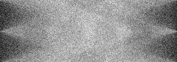
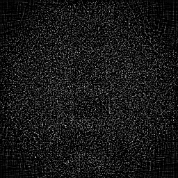
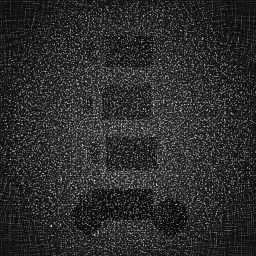
Experimental Setup — Signal Chain

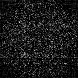
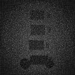
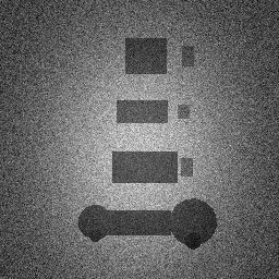
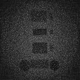
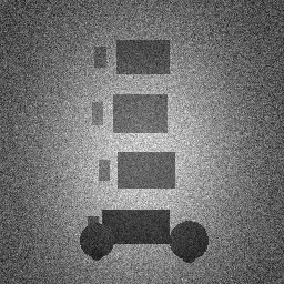
Reconstruction Gallery — 4 Scenes × 3 Scenarios
Method: CPU_baseline | Mismatch: nominal (nominal=True, perturbed=False)
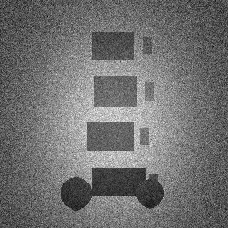
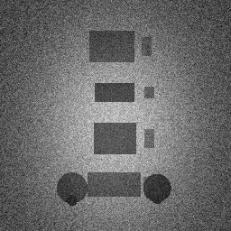
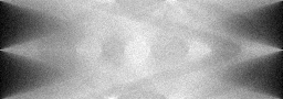
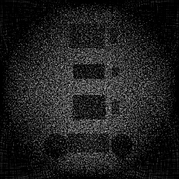
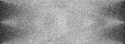
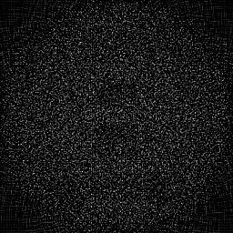
Ground Truth
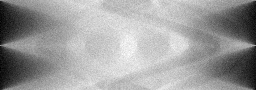
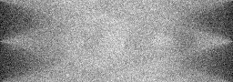
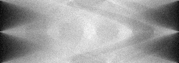
Measurement
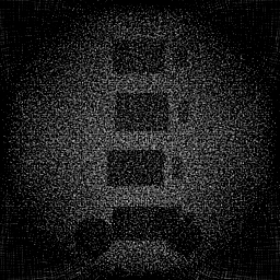
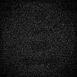
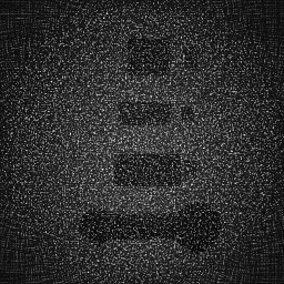
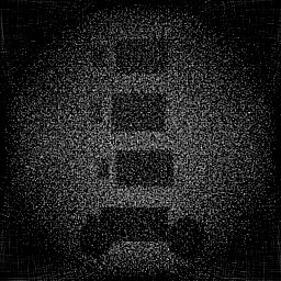
Reconstruction
Ground Truth
Measurement
Reconstruction
Ground Truth
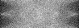
Measurement (perturbed)
Reconstruction

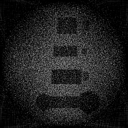
Mean PSNR Across All Scenes
Per-scene PSNR breakdown (4 scenes)
| Scene | I (PSNR) | I (SSIM) | II (PSNR) | II (SSIM) | III (PSNR) | III (SSIM) |
|---|---|---|---|---|---|---|
| scene_00 | 8.846315183602353 | 0.06783084626008488 | 8.087415147690969 | 0.024721298859753407 | 10.364036027938292 | 0.1590140264578491 |
| scene_01 | 9.90978722903076 | 0.07500519400245523 | 8.967564139192937 | 0.025167211948535956 | 11.436386690960978 | 0.1618398940991595 |
| scene_02 | 9.58168863560134 | 0.07454139108811705 | 8.613955033797208 | 0.02518255312462017 | 11.273283576754434 | 0.17073804162363052 |
| scene_03 | 8.983995765868114 | 0.07442520959756727 | 8.126370609310928 | 0.02457224644768539 | 10.34070091485338 | 0.15288025736778402 |
| Mean | 9.330446703525642 | 0.0729506602370561 | 8.44882623249801 | 0.024910827595148732 | 10.853601802626772 | 0.16111805488710576 |
Experimental Setup
Key References
- Blake & Fogelman, 'The role of DXA bone density scans in the diagnosis and treatment of osteoporosis', Postgrad. Med. J. 83, 509-517 (2007)
Canonical Datasets
- NHANES DXA reference data (CDC)
Spec DAG — Forward Model Pipeline
Λ(E₁,E₂) → Π(proj) → D(g, η₁)
Mismatch Parameters
| Symbol | Parameter | Description | Nominal | Perturbed |
|---|---|---|---|---|
| ΔE | energy_offset | Energy calibration offset (keV) | 0 | 1.0 |
| Δμ_s | soft_tissue | Soft-tissue attenuation error (%) | 0 | 3.0 |
| f_o | beam_overlap | Spectral overlap fraction | 0 | 0.02 |
Credits System
Spec Primitives Reference (11 primitives)
Free-space or medium propagation kernel (Fresnel, Rayleigh-Sommerfeld).
Spatial or spatio-temporal amplitude modulation (coded aperture, SLM pattern).
Geometric projection operator (Radon transform, fan-beam, cone-beam).
Sampling in the Fourier / k-space domain (MRI, ptychography).
Shift-invariant convolution with a point-spread function (PSF).
Summation along a physical dimension (spectral, temporal, angular).
Sensor readout with gain g and noise model η (Gaussian, Poisson, mixed).
Patterned illumination (block, Hadamard, random) applied to the scene.
Spectral dispersion element (prism, grating) with shift α and aperture a.
Sample or gantry rotation (CT, electron tomography).
Spectral filter or monochromator selecting a wavelength band.