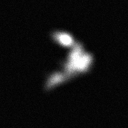
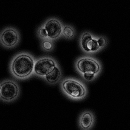
Confocal 3D
Confocal 3D Z-Stack
Standard reconstruction benchmark — forward model perfectly known, no calibration needed. Score = 0.5 × clip((PSNR−15)/30, 0, 1) + 0.5 × SSIM
| # | Method | Score | PSNR (dB) | SSIM | Source | |
|---|---|---|---|---|---|---|
| 🥇 |
DiffusionMicro
DiffusionMicro Gao 2024
39.9 dB
SSIM 0.963
Checkpoint unavailable
|
0.896 | 39.9 | 0.963 | ✓ Certified | Gao 2024 |
| 🥈 |
Restormer-3D
Restormer-3D Zamir 2022
38.6 dB
SSIM 0.951
Checkpoint unavailable
|
0.869 | 38.6 | 0.951 | ✓ Certified | Zamir 2022 |
| 🥉 |
SwinIR-3D
SwinIR-3D Liang 2021
37.5 dB
SSIM 0.942
Checkpoint unavailable
|
0.846 | 37.5 | 0.942 | ✓ Certified | Liang 2021 |
| 4 |
U-Net-3D
U-Net-3D Çiçek 2016
35.9 dB
SSIM 0.924
Checkpoint unavailable
|
0.810 | 35.9 | 0.924 | ✓ Certified | Çiçek 2016 |
| 5 |
CARE
CARE Weigert 2018
34.8 dB
SSIM 0.910
Checkpoint unavailable
|
0.785 | 34.8 | 0.910 | ✓ Certified | Weigert 2018 |
| 6 |
Noise2Void
Noise2Void Krull 2019
33.5 dB
SSIM 0.895
Checkpoint unavailable
|
0.756 | 33.5 | 0.895 | ✓ Certified | Krull 2019 |
| 7 | IRCNN-Confocal | 0.724 | 32.1 | 0.878 | ✓ Certified | Zhang 2017 |
| 8 | Wiener-3D | 0.639 | 28.5 | 0.828 | ✓ Certified | Wiener 1942 |
| 9 | Richardson-Lucy | 0.597 | 26.8 | 0.801 | ✓ Certified | Richardson 1972 |
Dataset: PWM Benchmark (9 algorithms)
Blind Reconstruction Challenge — forward model has unknown mismatch, must calibrate from data. Score = 0.4 × PSNR_norm + 0.4 × SSIM + 0.2 × (1 − ‖y − Ĥx̂‖/‖y‖)
| # | Method | Overall Score | Public PSNR / SSIM |
Dev PSNR / SSIM |
Hidden PSNR / SSIM |
Trust | Source |
|---|---|---|---|---|---|---|---|
| 🥇 | SwinIR-3D + gradient | 0.779 |
0.817
35.47 dB / 0.971
|
0.787
33.45 dB / 0.956
|
0.733
30.02 dB / 0.917
|
✓ Certified | Liang et al., ICCV 2021 (3D adapted) |
| 🥈 | DiffusionMicro + gradient | 0.771 |
0.844
37.28 dB / 0.979
|
0.765
31.85 dB / 0.941
|
0.705
27.93 dB / 0.879
|
✓ Certified | Gao et al., Nat. Methods 2024 |
| 🥉 | Restormer-3D + gradient | 0.767 |
0.851
37.5 dB / 0.980
|
0.759
31.6 dB / 0.938
|
0.690
27.88 dB / 0.878
|
✓ Certified | Zamir et al., CVPR 2022 (3D adapted) |
| 4 | IRCNN-Confocal + gradient | 0.711 |
0.740
29.69 dB / 0.912
|
0.729
29.53 dB / 0.909
|
0.665
27.21 dB / 0.863
|
✓ Certified | Zhang et al., CVPR 2017 |
| 5 | Noise2Void + gradient | 0.681 |
0.764
31.52 dB / 0.937
|
0.667
25.99 dB / 0.832
|
0.612
23.87 dB / 0.764
|
✓ Certified | Krull et al., CVPR 2019 |
| 6 | CARE + gradient | 0.680 |
0.781
32.73 dB / 0.950
|
0.679
26.78 dB / 0.853
|
0.580
23.37 dB / 0.745
|
✓ Certified | Weigert et al., Nat. Methods 2018 |
| 7 | U-Net-3D + gradient | 0.672 |
0.820
34.89 dB / 0.967
|
0.640
24.69 dB / 0.792
|
0.555
21.67 dB / 0.676
|
✓ Certified | Çiçek et al., MICCAI 2016 |
| 8 | Wiener-3D + gradient | 0.645 |
0.669
25.83 dB / 0.827
|
0.660
26.03 dB / 0.833
|
0.605
24.22 dB / 0.776
|
✓ Certified | Wiener, 1942 |
| 9 | Richardson-Lucy + gradient | 0.638 |
0.662
25.04 dB / 0.803
|
0.647
25.34 dB / 0.813
|
0.606
24.09 dB / 0.772
|
✓ Certified | Richardson, J. Opt. Soc. Am. 1972 |
Complete score requires all 3 tiers (Public + Dev + Hidden).
Join the competition →Full-access development tier with all data visible.
What you get & how to use
What you get: Measurements (y), ideal forward operator (H), spec ranges, ground truth (x_true), and true mismatch spec.
How to use: Load HDF5 → compare reconstruction vs x_true → check consistency → iterate.
What to submit: Reconstructed signals (x_hat) and corrected spec as HDF5.
Public Leaderboard
| # | Method | Score | PSNR | SSIM |
|---|---|---|---|---|
| 1 | Restormer-3D + gradient | 0.851 | 37.5 | 0.98 |
| 2 | DiffusionMicro + gradient | 0.844 | 37.28 | 0.979 |
| 3 | U-Net-3D + gradient | 0.820 | 34.89 | 0.967 |
| 4 | SwinIR-3D + gradient | 0.817 | 35.47 | 0.971 |
| 5 | CARE + gradient | 0.781 | 32.73 | 0.95 |
| 6 | Noise2Void + gradient | 0.764 | 31.52 | 0.937 |
| 7 | IRCNN-Confocal + gradient | 0.740 | 29.69 | 0.912 |
| 8 | Wiener-3D + gradient | 0.669 | 25.83 | 0.827 |
| 9 | Richardson-Lucy + gradient | 0.662 | 25.04 | 0.803 |
Spec Ranges (3 parameters)
| Parameter | Min | Max | Unit |
|---|---|---|---|
| z_step | -50.0 | 100.0 | nm |
| spherical_aberr | -0.1 | 0.2 | waves |
| refractive_index | 1.505 | 1.535 |
Blind evaluation tier — no ground truth available.
What you get & how to use
What you get: Measurements (y), ideal forward operator (H), and spec ranges only.
How to use: Apply your pipeline from the Public tier. Use consistency as self-check.
What to submit: Reconstructed signals and corrected spec. Scored server-side.
Dev Leaderboard
| # | Method | Score | PSNR | SSIM |
|---|---|---|---|---|
| 1 | SwinIR-3D + gradient | 0.787 | 33.45 | 0.956 |
| 2 | DiffusionMicro + gradient | 0.765 | 31.85 | 0.941 |
| 3 | Restormer-3D + gradient | 0.759 | 31.6 | 0.938 |
| 4 | IRCNN-Confocal + gradient | 0.729 | 29.53 | 0.909 |
| 5 | CARE + gradient | 0.679 | 26.78 | 0.853 |
| 6 | Noise2Void + gradient | 0.667 | 25.99 | 0.832 |
| 7 | Wiener-3D + gradient | 0.660 | 26.03 | 0.833 |
| 8 | Richardson-Lucy + gradient | 0.647 | 25.34 | 0.813 |
| 9 | U-Net-3D + gradient | 0.640 | 24.69 | 0.792 |
Spec Ranges (3 parameters)
| Parameter | Min | Max | Unit |
|---|---|---|---|
| z_step | -60.0 | 90.0 | nm |
| spherical_aberr | -0.12 | 0.18 | waves |
| refractive_index | 1.503 | 1.533 |
Fully blind server-side evaluation — no data download.
What you get & how to use
What you get: No data downloadable. Algorithm runs server-side on hidden measurements.
How to use: Package algorithm as Docker container / Python script. Submit via link.
What to submit: Containerized algorithm accepting y + H, outputting x_hat + corrected spec.
Hidden Leaderboard
| # | Method | Score | PSNR | SSIM |
|---|---|---|---|---|
| 1 | SwinIR-3D + gradient | 0.733 | 30.02 | 0.917 |
| 2 | DiffusionMicro + gradient | 0.705 | 27.93 | 0.879 |
| 3 | Restormer-3D + gradient | 0.690 | 27.88 | 0.878 |
| 4 | IRCNN-Confocal + gradient | 0.665 | 27.21 | 0.863 |
| 5 | Noise2Void + gradient | 0.612 | 23.87 | 0.764 |
| 6 | Richardson-Lucy + gradient | 0.606 | 24.09 | 0.772 |
| 7 | Wiener-3D + gradient | 0.605 | 24.22 | 0.776 |
| 8 | CARE + gradient | 0.580 | 23.37 | 0.745 |
| 9 | U-Net-3D + gradient | 0.555 | 21.67 | 0.676 |
Spec Ranges (3 parameters)
| Parameter | Min | Max | Unit |
|---|---|---|---|
| z_step | -35.0 | 115.0 | nm |
| spherical_aberr | -0.07 | 0.23 | waves |
| refractive_index | 1.508 | 1.538 |
Blind Reconstruction Challenge
ChallengeGiven measurements with unknown mismatch and spec ranges (not exact params), reconstruct the original signal. A method must be evaluated on all three tiers for a complete score. Scored on a composite metric: 0.4 × PSNR_norm + 0.4 × SSIM + 0.2 × (1 − ‖y − Ĥx̂‖/‖y‖).
Measurements y, ideal forward model H, spec ranges
Reconstructed signal x̂
About the Imaging Modality
Three-dimensional confocal imaging by acquiring a z-stack of optical sections. Each slice is convolved with the 3D confocal PSF. The anisotropic PSF (axial resolution ~3x worse than lateral) is a key challenge. 3D Richardson-Lucy or CARE-3D are used for volumetric deconvolution. The forward model is y(x,y,z) = PSF_3d *** x(x,y,z) + n where *** denotes 3D convolution.
Principle
Same confocal principle as live-cell mode but acquiring a full z-stack by stepping the objective or sample through the focal plane. Each optical section is convolved with the 3-D confocal PSF, and the full volume is reconstructed by 3-D deconvolution to recover isotropic resolution.
How to Build the System
Use a high-NA objective (60-100x, 1.4 NA oil or 1.2 NA water) with a piezo z-stage for precise, repeatable z-steps (typ. 200-300 nm). Acquire z-stacks covering the specimen thickness with Nyquist z-sampling. For fixed samples, oil immersion is preferred; for thick tissue, use silicone oil or glycerol objectives to minimize RI mismatch deep in the sample.
Common Reconstruction Algorithms
- 3-D Richardson-Lucy deconvolution
- 3-D Wiener / Tikhonov deconvolution
- Huygens Professional iterative deconvolution
- DeconvolutionLab2 (GPU-accelerated 3-D)
- Deep-learning volumetric restoration (3-D U-Net, RCAN3D)
Common Mistakes
- Using z-step larger than Nyquist, causing axial aliasing
- Depth-dependent spherical aberration from RI mismatch not corrected
- Not accounting for signal attenuation deeper in the sample
- Applying 2-D deconvolution slice-by-slice instead of full 3-D
- Incorrect PSF model (2-D Gaussian instead of 3-D Born & Wolf model)
How to Avoid Mistakes
- Calculate Nyquist z-step (λ / (4·n·(1-cos α))) and sample accordingly
- Use depth-dependent PSF models or adaptive optics for thick specimens
- Apply intensity normalization per z-slice before deconvolution
- Always perform true 3-D deconvolution to preserve axial information
- Use measured 3-D PSF from sub-diffraction beads embedded at the correct depth
Forward-Model Mismatch Cases
- The widefield fallback processes only 2D (64,64) images, but confocal 3D requires volumetric input (32,64,64) — the entire z-stack is discarded, losing all axial information
- Applying 2D deconvolution slice-by-slice instead of true 3D deconvolution produces incorrect axial resolution and misses inter-slice correlations from the 3D PSF
How to Correct the Mismatch
- Use the 3D confocal operator that processes full z-stack volumes with the anisotropic 3D PSF (worse axial than lateral resolution)
- Perform true 3D deconvolution using the measured or modeled 3D confocal PSF; never decompose a z-stack into independent 2D slices
Experimental Setup — Signal Chain

Reconstruction Gallery — 4 Scenes × 3 Scenarios
Method: CPU_baseline | Mismatch: nominal (nominal=True, perturbed=False)

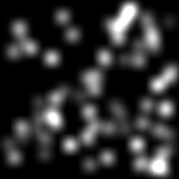
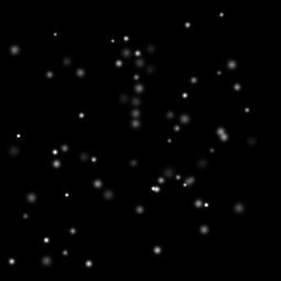
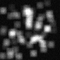
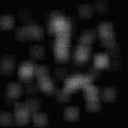
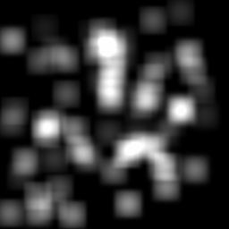
Ground Truth
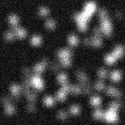
Measurement
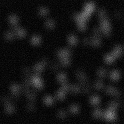
Reconstruction
Ground Truth
Measurement

Reconstruction
Ground Truth
Measurement (perturbed)
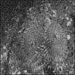
Reconstruction


Mean PSNR Across All Scenes
Per-scene PSNR breakdown (4 scenes)
| Scene | I (PSNR) | I (SSIM) | II (PSNR) | II (SSIM) | III (PSNR) | III (SSIM) |
|---|---|---|---|---|---|---|
| scene_00 | 17.886302732164115 | 0.01892072832102963 | 17.7485439802784 | 0.009289703811224622 | 8.402567163839525 | 0.003161693395142872 |
| scene_01 | 22.783144034430713 | 0.3272043062993476 | 20.414571235543796 | 0.14551700775883114 | 8.58243391232876 | 0.001742691581889463 |
| scene_02 | 22.25307857472778 | 0.5892049547357852 | 16.286545577941986 | 0.37585323583290936 | 5.619616483931034 | 0.01167634410824235 |
| scene_03 | 17.27371209222946 | 0.043762909709512604 | 15.907989100545086 | 0.021283995651325983 | 5.600425139556533 | 0.0031946534455390965 |
| Mean | 20.049059358388018 | 0.24477322476641875 | 17.589412473577315 | 0.1379859857635728 | 7.051260674913962 | 0.004943845632703446 |
Experimental Setup
Key References
- McNally et al., 'Three-dimensional imaging by deconvolution microscopy', Methods 23, 210-217 (1999)
- Weigert et al., 'Isotropic reconstruction of 3D fluorescence microscopy images using convolutional neural networks', MICCAI 2017
Canonical Datasets
- Planaria 3D confocal dataset (Weigert et al.)
- BioSR confocal 3D subset
Spec DAG — Forward Model Pipeline
C(PSF_3D) → D(g, η₃)
Mismatch Parameters
| Symbol | Parameter | Description | Nominal | Perturbed |
|---|---|---|---|---|
| Δz | z_step | Z-step size error (nm) | 0 | 50 |
| C_s | spherical_aberr | Spherical aberration (waves) | 0 | 0.1 |
| Δn | refractive_index | Refractive index mismatch | 1.515 | 1.525 |
Credits System
Spec Primitives Reference (11 primitives)
Free-space or medium propagation kernel (Fresnel, Rayleigh-Sommerfeld).
Spatial or spatio-temporal amplitude modulation (coded aperture, SLM pattern).
Geometric projection operator (Radon transform, fan-beam, cone-beam).
Sampling in the Fourier / k-space domain (MRI, ptychography).
Shift-invariant convolution with a point-spread function (PSF).
Summation along a physical dimension (spectral, temporal, angular).
Sensor readout with gain g and noise model η (Gaussian, Poisson, mixed).
Patterned illumination (block, Hadamard, random) applied to the scene.
Spectral dispersion element (prism, grating) with shift α and aperture a.
Sample or gantry rotation (CT, electron tomography).
Spectral filter or monochromator selecting a wavelength band.