CASSI
Coded Aperture Snapshot Spectral Imaging
Standard reconstruction benchmark — forward model perfectly known, no calibration needed. Score = 0.5 × clip((PSNR−15)/30, 0, 1) + 0.5 × SSIM
| # | Method | Score | PSNR (dB) | SSIM | Source | |
|---|---|---|---|---|---|---|
| 🥇 | MiJUN-5stg | 0.927 | 40.9 | 0.991 | ✓ Certified | Meng et al. AAAI 2025 |
| 🥈 | RDLUF-MixS2-9stg | 0.904 | 39.6 | 0.988 | ✓ Certified | Dong et al. CVPR 2023 |
| 🥉 | DAUHST-9stg | 0.883 | 38.4 | 0.985 | ✓ Certified | Cai et al. NeurIPS 2022 |
| 4 | PADUT-3stg | 0.854 | 36.95 | 0.975 | ✓ Certified | Li et al. ICCV 2023 |
| 5 | CST-L-Plus | 0.836 | 36.1 | 0.967 | ✓ Certified | Cai et al. ECCV 2022 |
| 6 | MST++ | 0.833 | 36.0 | 0.966 | ✓ Certified | Cai et al. CVPRW 2022 |
| 7 | MST-L | 0.809 | 34.81 | 0.958 | ✓ Certified | Cai et al. CVPR 2022 |
| 8 | HDNet | 0.804 | 34.66 | 0.952 | ✓ Certified | Hu et al. CVPR 2022 |
| 9 | SSR-L | 0.797 | 34.0 | 0.960 | ✓ Certified | Zhang et al. CVPR 2024 |
| 10 | DGSMP | 0.752 | 32.6 | 0.917 | ✓ Certified | Huang et al. CVPR 2021 |
| 11 | TSA-Net | 0.722 | 31.5 | 0.894 | ✓ Certified | Meng et al. ECCV 2020 |
| 12 | λ-Net | 0.696 | 30.1 | 0.887 | ✓ Certified | Miao et al. ICCV 2019 |
| 13 | BIRNAT | 0.694 | 30.0 | 0.887 | ✓ Certified | Cheng et al. ECCV 2022 |
| 14 | ADMM-Net | 0.674 | 29.1 | 0.877 | ✓ Certified | Ma et al. ICCV 2019 |
| 15 | GAP-Net | 0.669 | 29.1 | 0.867 | ✓ Certified | Meng et al. 2020 |
| 16 | GAP-TV | 0.577 | 24.34 | 0.820 | ✓ Certified | Yuan et al. 2016 |
| 17 | PnP-HSICNN | 0.573 | 25.12 | 0.810 | ✓ Certified | Maffei et al. 2020 |
| 18 | TwIST | 0.538 | 23.1 | 0.800 | ✓ Certified | Bioucas-Dias & Figueiredo 2007 |
Dataset: KAIST simu, 256×256×28
Blind Reconstruction Challenge — forward model has unknown mismatch, must calibrate from data. Score = 0.4 × PSNR_norm + 0.4 × SSIM + 0.2 × (1 − ‖y − Ĥx̂‖/‖y‖)
| # | Method | Overall Score | Public PSNR / SSIM |
Dev PSNR / SSIM |
Hidden PSNR / SSIM |
Trust | Source |
|---|---|---|---|---|---|---|---|
| 🥇 | SSR-L + gradient | 0.626 |
0.877
38.03 dB / 0.994
|
0.545
19.53 dB / 0.626
|
0.456
17.06 dB / 0.473
|
✓ Certified | PWM benchmark (CVPR 2024) |
| 🥈 | GAP-TV + gradient | 0.593 |
0.687
24.21 dB / 0.865
|
0.576
19.69 dB / 0.699
|
0.516
18.37 dB / 0.583
|
✓ Certified | PWM benchmark |
| 🥉 | MST-L + gradient | 0.550 |
0.794
31.29 dB / 0.977
|
0.472
17.18 dB / 0.550
|
0.385
15.45 dB / 0.384
|
✓ Certified | PWM benchmark |
| 4 | PnP-HSICNN + gradient | 0.504 |
0.549
20.06 dB / 0.675
|
0.508
16.88 dB / 0.621
|
0.455
15.59 dB / 0.518
|
✓ Certified | PWM benchmark |
| 5 | HDNet + gradient | 0.439 |
0.707
25.45 dB / 0.921
|
0.329
13.59 dB / 0.427
|
0.280
10.96 dB / 0.373
|
✓ Certified | PWM benchmark |
Complete score requires all 3 tiers (Public + Dev + Hidden).
Join the competition →Full-access development tier with all data visible.
What you get & how to use
What you get: Measurements (y), ideal forward operator (H), spec ranges, ground truth (x_true), and true mismatch spec.
How to use: Load HDF5 → compare reconstruction vs x_true → check consistency → iterate.
What to submit: Reconstructed signals (x_hat) and corrected spec as HDF5.
Public Leaderboard
| # | Method | Score | PSNR | SSIM |
|---|---|---|---|---|
| 1 | SSR-L + gradient | 0.877 | 38.03 | 0.994 |
| 2 | MST-L + gradient | 0.794 | 31.29 | 0.977 |
| 3 | HDNet + gradient | 0.707 | 25.45 | 0.921 |
| 4 | GAP-TV + gradient | 0.687 | 24.21 | 0.865 |
| 5 | PnP-HSICNN + gradient | 0.549 | 20.06 | 0.675 |
Spec Ranges (5 parameters)
| Parameter | Min | Max | Unit |
|---|---|---|---|
| mask_dx | 0.3 | 0.7 | px |
| mask_dy | 0.1 | 0.5 | px |
| mask_rotation | 0.0 | 0.2 | deg |
| dispersion_slope | 1.895 | 2.145 | px/band |
| dispersion_axis | 0.0 | 0.3 | deg |
Blind evaluation tier — no ground truth available.
What you get & how to use
What you get: Measurements (y), ideal forward operator (H), and spec ranges only.
How to use: Apply your pipeline from the Public tier. Use consistency as self-check.
What to submit: Reconstructed signals and corrected spec. Scored server-side.
Dev Leaderboard
| # | Method | Score | PSNR | SSIM |
|---|---|---|---|---|
| 1 | GAP-TV + gradient | 0.576 | 19.69 | 0.699 |
| 2 | SSR-L + gradient | 0.545 | 19.53 | 0.626 |
| 3 | PnP-HSICNN + gradient | 0.508 | 16.88 | 0.621 |
| 4 | MST-L + gradient | 0.472 | 17.18 | 0.55 |
| 5 | HDNet + gradient | 0.329 | 13.59 | 0.427 |
Spec Ranges (5 parameters)
| Parameter | Min | Max | Unit |
|---|---|---|---|
| mask_dx | 0.4 | 0.8 | px |
| mask_dy | 0.2 | 0.6 | px |
| mask_rotation | 0.05 | 0.25 | deg |
| dispersion_slope | 1.825 | 2.075 | px/band |
| dispersion_axis | 0.07 | 0.37 | deg |
Fully blind server-side evaluation — no data download.
What you get & how to use
What you get: No data downloadable. Algorithm runs server-side on hidden measurements.
How to use: Package algorithm as Docker container / Python script. Submit via link.
What to submit: Containerized algorithm accepting y + H, outputting x_hat + corrected spec.
Hidden Leaderboard
| # | Method | Score | PSNR | SSIM |
|---|---|---|---|---|
| 1 | GAP-TV + gradient | 0.516 | 18.37 | 0.583 |
| 2 | SSR-L + gradient | 0.456 | 17.06 | 0.473 |
| 3 | PnP-HSICNN + gradient | 0.455 | 15.59 | 0.518 |
| 4 | MST-L + gradient | 0.385 | 15.45 | 0.384 |
| 5 | HDNet + gradient | 0.280 | 10.96 | 0.373 |
Spec Ranges (5 parameters)
| Parameter | Min | Max | Unit |
|---|---|---|---|
| mask_dx | 0.2 | 0.6 | px |
| mask_dy | 0.0 | 0.4 | px |
| mask_rotation | -0.05 | 0.15 | deg |
| dispersion_slope | 1.955 | 2.205 | px/band |
| dispersion_axis | -0.05 | 0.25 | deg |
Blind Reconstruction Challenge
ChallengeGiven measurements with unknown mismatch and spec ranges (not exact params), reconstruct the original signal. A method must be evaluated on all three tiers for a complete score. Scored on a composite metric: 0.4 × PSNR_norm + 0.4 × SSIM + 0.2 × (1 − ‖y − Ĥx̂‖/‖y‖).
Measurements y, ideal forward model H, spec ranges
Reconstructed signal x̂
About the Imaging Modality
CASSI captures a 3D hyperspectral data cube (2 spatial + 1 spectral dimension) in a single 2D camera exposure. The scene is modulated by a binary coded aperture mask, spectrally dispersed by a prism, and integrated onto a 2D detector. The forward model is y = H*x + n where H encodes both coded-aperture modulation and spectral-dispersion shift. Compression ratios equal the number of spectral bands (e.g. 28:1). Reconstruction exploits spectral correlation via GAP-TV, MST, or CST.
Principle
Coded Aperture Snapshot Spectral Imaging (CASSI) captures a full 3-D spectral datacube (x, y, λ) in a single 2-D snapshot by encoding the scene with a binary coded aperture and spectrally dispersing it with a prism onto the detector. Different spectral channels are shifted and superimposed on the sensor, creating a compressed measurement. Computational algorithms recover the full datacube from this single measurement using sparsity priors.
How to Build the System
Build an optical relay with an objective lens, place a binary coded aperture (lithographic chrome-on-glass mask or DMD) at an intermediate image plane, then disperse with an Amici or double-Amici prism, and re-image onto a high-resolution detector (2048× 2048+ pixels). Precisely calibrate the spectral dispersion curve (nm/pixel). The coded aperture pattern should have ~50 % transmittance and good conditioning.
Common Reconstruction Algorithms
- TwIST (Two-step Iterative Shrinkage/Thresholding)
- GAP-TV (Generalized Alternating Projection with Total Variation)
- ADMM with sparsity in DCT or wavelet domain
- Deep unfolding networks (DGSMP, TSA-Net, BIRNAT)
- Plug-and-Play ADMM with learned denoisers
Common Mistakes
- Poor spectral calibration causing wavelength assignment errors across the datacube
- Coded aperture not precisely at the image plane, blurring the code modulation
- Insufficient detector resolution relative to the number of spectral bands
- Ignoring optical aberrations in the dispersive relay that vary with wavelength
- Using a random mask without checking its sensing matrix condition number
How to Avoid Mistakes
- Calibrate spectral mapping with monochromatic sources at known wavelengths
- Mount coded aperture on a precision z-stage and focus to maximize modulation contrast
- Ensure detector pixel count > (spatial pixels × spectral bands) for adequate compression ratio
- Design the relay optics for uniform imaging quality across the spectral range
- Optimize or simulate the mask pattern for low coherence (good RIP) before fabrication
Forward-Model Mismatch Cases
- The widefield fallback produces a 2D (64,64) grayscale image, but CASSI compresses a 3D spectral datacube (64,64,L wavelengths) into a single 2D coded snapshot via a binary mask and dispersive prism — the spectral dimension is entirely absent
- Without the coded aperture mask and spectral dispersion, the measurement does not encode wavelength-dependent information — spectral unmixing or hyperspectral reconstruction from the fallback output is impossible
How to Correct the Mismatch
- Use the CASSI operator that applies the binary coded aperture mask followed by spectral dispersion (prism/grating shift), producing a 2D coded measurement that encodes the full 3D spectral datacube
- Reconstruct the (x,y,lambda) datacube using compressive sensing (TwIST, GAP-TV) or deep unfolding networks (TSA-Net, MST) that exploit the spatio-spectral structure encoded by the CASSI forward model
Experimental Setup — Signal Chain

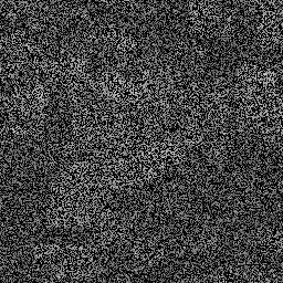
Reconstruction Gallery — 4 Scenes × 3 Scenarios
Method: CPU_baseline | Mismatch: nominal (nominal=True, perturbed=False)
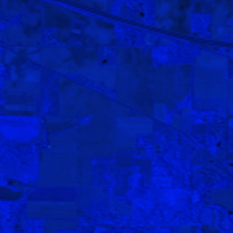
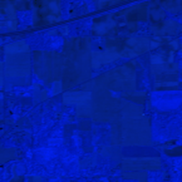
Ground Truth

Measurement
Reconstruction
Ground Truth

Measurement
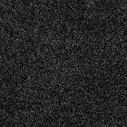
Reconstruction
Ground Truth
Measurement (perturbed)
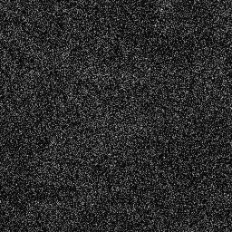
Reconstruction


Mean PSNR Across All Scenes
Per-scene PSNR breakdown (4 scenes)
| Scene | I (PSNR) | I (SSIM) | II (PSNR) | II (SSIM) | III (PSNR) | III (SSIM) |
|---|---|---|---|---|---|---|
| scene_00 | 11.388157370414833 | 0.01733572164482545 | 16.29034469671149 | 0.04138063796264847 | 16.419408068168842 | 0.045509048931950055 |
| scene_01 | 11.604006893341834 | 0.01871242508822704 | 16.262318979148382 | 0.041985050757947055 | 16.342202770675012 | 0.045774250082260305 |
| scene_02 | 11.332959495650615 | 0.01710600322887299 | 16.354152003784925 | 0.043263103647925995 | 16.27598154571157 | 0.04582825340291557 |
| scene_03 | 11.9781210538936 | 0.01968244532966781 | 16.251118459587204 | 0.04159571449035334 | 16.38499506997022 | 0.04578811472898349 |
| Mean | 11.575811203325221 | 0.018209148822898324 | 16.289483534808 | 0.042056126714718714 | 16.35564686363141 | 0.04572491678652736 |
Experimental Setup
Key References
- Wagadarikar et al., 'Single disperser design for coded aperture snapshot spectral imaging', Applied Optics 47, B44-B51 (2008)
- Cai et al., 'Mask-guided Spectral-wise Transformer (MST++)', CVPRW 2022
Canonical Datasets
- CAVE (Columbia, 32 scenes, 512x512x31)
- KAIST (30 scenes, 2704x3376x28)
- ARAD_1K (1000 hyperspectral images)
Spec DAG — Forward Model Pipeline
M(mask) → W(α, a) → Σ_λ → D(g, η₄)
Mismatch Parameters
| Symbol | Parameter | Description | Nominal | Perturbed |
|---|---|---|---|---|
| Δx | mask_dx | Mask lateral shift (pixels) | 0 | 0.5 |
| Δy | mask_dy | Mask vertical shift (pixels) | 0 | 0.3 |
| θ | mask_theta | Mask rotation (rad) | 0 | 0.1 |
| a₁ | disp_a1 | Dispersion coefficient | 2.0 | 2.02 |
| α | disp_alpha | Dispersion angle (rad) | 0 | 0.15 |
| σ_r | sigma_read | Detector read noise std (electrons) | 5.0 | 8.0 |
| I_d | dark_current | Dark current (electrons/pixel/s) | 0.1 | 0.5 |
| g | gain | Detector gain multiplier | 1.0 | 1.03 |
Credits System
Spec Primitives Reference (11 primitives)
Free-space or medium propagation kernel (Fresnel, Rayleigh-Sommerfeld).
Spatial or spatio-temporal amplitude modulation (coded aperture, SLM pattern).
Geometric projection operator (Radon transform, fan-beam, cone-beam).
Sampling in the Fourier / k-space domain (MRI, ptychography).
Shift-invariant convolution with a point-spread function (PSF).
Summation along a physical dimension (spectral, temporal, angular).
Sensor readout with gain g and noise model η (Gaussian, Poisson, mixed).
Patterned illumination (block, Hadamard, random) applied to the scene.
Spectral dispersion element (prism, grating) with shift α and aperture a.
Sample or gantry rotation (CT, electron tomography).
Spectral filter or monochromator selecting a wavelength band.