CACTI
Coded Aperture Compressive Temporal Imaging
Standard reconstruction benchmark — forward model perfectly known, no calibration needed. Score = 0.5 × clip((PSNR−15)/30, 0, 1) + 0.5 × SSIM
| # | Method | Score | PSNR (dB) | SSIM | Source | |
|---|---|---|---|---|---|---|
| 🥇 | HiSViT-9 | 0.876 | 38.24 | 0.978 | ✓ Certified | HiSViT (ECCV 2024) |
| 🥈 | EfficientSCI | 0.867 | 37.71 | 0.976 | ✓ Certified | EfficientSCI (CVPR 2023) |
| 🥉 | ELP-Unfolding | 0.826 | 35.54 | 0.968 | ✓ Certified | ELP-Unfolding (2022) |
| 4 | RevSCI | 0.786 | 33.49 | 0.956 | ✓ Certified | RevSCI (TPAMI 2022) |
| 5 | BIRNAT | 0.715 | 30.26 | 0.921 | ✓ Certified | BIRNAT (TPAMI 2021) |
| 6 | GAP-TV | 0.630 | 26.02 | 0.892 | ✓ Certified | GAP-TV (Signal Processing 2016) |
Dataset: 6-scene simulation, T=8, Cr=8
Blind Reconstruction Challenge — forward model has unknown mismatch, must calibrate from data. Score = 0.4 × PSNR_norm + 0.4 × SSIM + 0.2 × (1 − ‖y − Ĥx̂‖/‖y‖)
| # | Method | Overall Score | Public PSNR / SSIM |
Dev PSNR / SSIM |
Hidden PSNR / SSIM |
Trust | Source |
|---|---|---|---|---|---|---|---|
| 🥇 |
ELP-Unfolding + blind cal
ELP-Unfolding + blind cal InverseNet Scenario IV (blind cal, improved hybrid grid search) Score 0.191
Correct & Reconstruct →
|
0.191 |
0.572
23.06 dB / 0.672
|
— | — | ✓ Certified | InverseNet Scenario IV (blind cal, improved hybrid grid search) |
| 🥈 |
EfficientSCI + blind cal
EfficientSCI + blind cal InverseNet Scenario IV (blind cal, improved hybrid grid search) Score 0.189
Correct & Reconstruct →
|
0.189 |
0.567
22.65 dB / 0.676
|
— | — | ✓ Certified | InverseNet Scenario IV (blind cal, improved hybrid grid search) |
| 🥉 |
HiSViT-9 + blind cal
HiSViT-9 + blind cal InverseNet Scenario IV (blind cal, improved hybrid grid search) Score 0.188
Correct & Reconstruct →
|
0.188 |
0.565
22.58 dB / 0.673
|
— | — | ✓ Certified | InverseNet Scenario IV (blind cal, improved hybrid grid search) |
| 4 |
GAP-TV + blind cal
GAP-TV + blind cal InverseNet Scenario IV (blind cal, improved hybrid grid search) Score 0.174
Correct & Reconstruct →
|
0.174 |
0.522
21.79 dB / 0.590
|
— | — | ✓ Certified | InverseNet Scenario IV (blind cal, improved hybrid grid search) |
| 5 |
PnP-FFDNet + blind cal
PnP-FFDNet + blind cal InverseNet Scenario IV (blind cal, improved hybrid grid search) Score 0.149
Correct & Reconstruct →
|
0.149 |
0.446
17.37 dB / 0.542
|
— | — | ✓ Certified | InverseNet Scenario IV (blind cal, improved hybrid grid search) |
Complete score requires all 3 tiers (Public + Dev + Hidden).
Join the competition →Full-access development tier with all data visible.
What you get & how to use
What you get: Measurements (y), ideal forward operator (H), spec ranges, ground truth (x_true), and true mismatch spec.
How to use: Load HDF5 → compare reconstruction vs x_true → check consistency → iterate.
What to submit: Reconstructed signals (x_hat) and corrected spec as HDF5.
Public Leaderboard
| # | Method | Score | PSNR | SSIM |
|---|---|---|---|---|
| 1 | ELP-Unfolding + blind cal | 0.572 | 23.06 | 0.672 |
| 2 | EfficientSCI + blind cal | 0.567 | 22.65 | 0.676 |
| 3 | HiSViT-9 + blind cal | 0.565 | 22.58 | 0.673 |
| 4 | GAP-TV + blind cal | 0.522 | 21.79 | 0.59 |
| 5 | PnP-FFDNet + blind cal | 0.446 | 17.37 | 0.542 |
Spec Ranges (7 parameters)
| Parameter | Min | Max | Unit |
|---|---|---|---|
| mask_dx | 0.2 | 0.8 | px |
| mask_dy | 0.1 | 0.5 | px |
| mask_rotation | -0.05 | 0.25 | deg |
| mask_blur | -0.25 | 0.25 | px |
| clock_offset | -0.05 | 0.15 | frames |
| gain_drift | 0.97 | 1.07 | |
| offset_drift | -0.018 | 0.022 |
Blind evaluation tier — no ground truth available.
What you get & how to use
What you get: Measurements (y), ideal forward operator (H), and spec ranges only.
How to use: Apply your pipeline from the Public tier. Use consistency as self-check.
What to submit: Reconstructed signals and corrected spec. Scored server-side.
Dev Leaderboard
| # | Method | Score | PSNR | SSIM |
|---|---|---|---|---|
| 1 | ELP-Unfolding + blind cal | 0.000 | 0.0 | 0.0 |
| 2 | EfficientSCI + blind cal | 0.000 | 0.0 | 0.0 |
| 3 | HiSViT-9 + blind cal | 0.000 | 0.0 | 0.0 |
| 4 | GAP-TV + blind cal | 0.000 | 0.0 | 0.0 |
| 5 | PnP-FFDNet + blind cal | 0.000 | 0.0 | 0.0 |
Spec Ranges (7 parameters)
| Parameter | Min | Max | Unit |
|---|---|---|---|
| mask_dx | 0.05 | 0.65 | px |
| mask_dy | 0.0 | 0.4 | px |
| mask_rotation | -0.07 | 0.23 | deg |
| mask_blur | -0.15 | 0.35 | px |
| clock_offset | -0.13 | 0.07 | frames |
| gain_drift | 0.93 | 1.03 | |
| offset_drift | -0.03 | 0.01 |
Fully blind server-side evaluation — no data download.
What you get & how to use
What you get: No data downloadable. Algorithm runs server-side on hidden measurements.
How to use: Package algorithm as Docker container / Python script. Submit via link.
What to submit: Containerized algorithm accepting y + H, outputting x_hat + corrected spec.
Hidden Leaderboard
| # | Method | Score | PSNR | SSIM |
|---|---|---|---|---|
| 1 | ELP-Unfolding + blind cal | 0.000 | 0.0 | 0.0 |
| 2 | EfficientSCI + blind cal | 0.000 | 0.0 | 0.0 |
| 3 | HiSViT-9 + blind cal | 0.000 | 0.0 | 0.0 |
| 4 | GAP-TV + blind cal | 0.000 | 0.0 | 0.0 |
| 5 | PnP-FFDNet + blind cal | 0.000 | 0.0 | 0.0 |
Spec Ranges (7 parameters)
| Parameter | Min | Max | Unit |
|---|---|---|---|
| mask_dx | 0.35 | 0.95 | px |
| mask_dy | 0.2 | 0.6 | px |
| mask_rotation | 0.07 | 0.37 | deg |
| mask_blur | 0.1 | 0.6 | px |
| clock_offset | -0.02 | 0.18 | frames |
| gain_drift | 0.99 | 1.09 | |
| offset_drift | -0.005 | 0.035 |
Blind Reconstruction Challenge
ChallengeGiven measurements with unknown mismatch and spec ranges (not exact params), reconstruct the original signal. A method must be evaluated on all three tiers for a complete score. Scored on a composite metric: 0.4 × PSNR_norm + 0.4 × SSIM + 0.2 × (1 − ‖y − Ĥx̂‖/‖y‖).
Measurements y, ideal forward model H, spec ranges
Reconstructed signal x̂
About the Imaging Modality
CACTI captures multiple video frames in a single camera exposure by modulating the scene with a shifting binary mask during the integration period. Each temporal frame sees a different mask pattern, and the detector integrates all modulated frames into a single 2D measurement. The forward model is y = sum_t M_t * x_t + n where M_t is the mask at time t. Typical compression ratios are 8-48 frames per snapshot. Reconstruction exploits temporal correlation via GAP-TV, PnP-FFDNet, or deep unfolding networks (STFormer, EfficientSCI).
Principle
Coded Aperture Compressive Temporal Imaging (CACTI) compresses multiple high-speed video frames into a single sensor exposure by modulating the scene with a dynamic coded aperture (shifting mask) during the integration time. The sensor accumulates a coded sum of B consecutive frames, and computational algorithms recover all B frames from the single compressed measurement using video sparsity priors.
How to Build the System
Build a relay optical system with a physical translating mask or use a DMD as the coded aperture at an intermediate image plane. The mask shifts by one pixel per sub-frame interval during the camera integration time, effectively encoding B temporal frames. Use a standard camera at normal frame rate (e.g., 30 fps) to capture the compressed measurement. Calibrate the mask pattern and its motion precisely.
Common Reconstruction Algorithms
- GAP-TV (Generalized Alternating Projection with Total Variation)
- DeSCI (Decompress Snapshot Compressive Imaging, GMM prior)
- PnP-FFDNet (Plug-and-Play with FFDNet denoiser)
- Deep unfolding: BIRNAT, RevSCI, EfficientSCI
- E2E-trained networks: STFormer, CST (transformer-based)
Common Mistakes
- Mask calibration error causing temporal frame misalignment in reconstruction
- Compression ratio too high (too many sub-frames per snapshot) for the scene motion
- Motion blur within individual sub-frame intervals when scene moves fast
- Non-uniform mask illumination creating brightness gradients in recovered frames
- Choosing masks with poor conditioning (high mutual coherence between rows)
How to Avoid Mistakes
- Calibrate mask position precisely using a static known pattern before experiments
- Limit compression ratio (B ≤ 8-10 for complex natural scenes; B ≤ 24-48 for simpler scenes)
- Ensure sub-frame exposure is short enough that intra-frame motion is negligible
- Flatfield-correct the mask modulation using a uniform target calibration
- Simulate reconstruction quality with candidate mask patterns before hardware fabrication
Forward-Model Mismatch Cases
- The widefield fallback processes a single 2D (64,64) frame, but CACTI compresses B temporal frames into a single 2D coded snapshot using a shifting binary mask — the temporal dimension (64,64,B) is entirely lost
- Without the time-varying coded exposure pattern, individual video frames cannot be separated from the compressed measurement — temporal super-resolution from the fallback is impossible
How to Correct the Mismatch
- Use the CACTI operator that applies frame-wise binary masks and sums the coded frames: y = sum_b(M_b * x_b), compressing B frames into one measurement
- Reconstruct the video sequence using PnP-SCI (plug-and-play with FastDVDnet), ELP-Unfolding, or GAP-TV that model the temporal compression and recover B frames from the single snapshot
Experimental Setup — Signal Chain

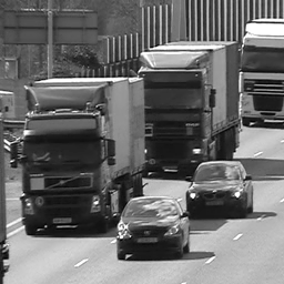
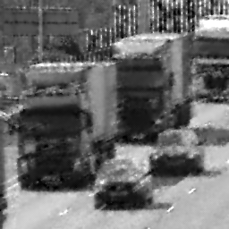
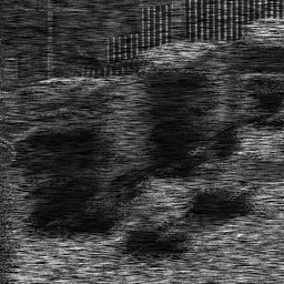
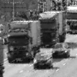
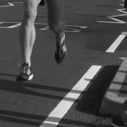
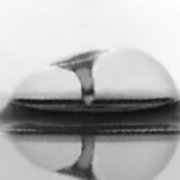
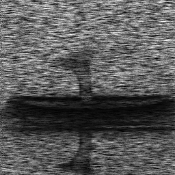
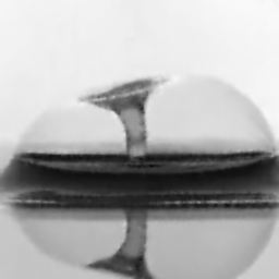
Reconstruction Gallery — 4 Scenes × 3 Scenarios
Method: CPU_baseline | Mismatch: nominal (nominal=True, perturbed=False)
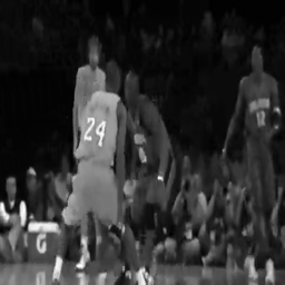
Ground Truth
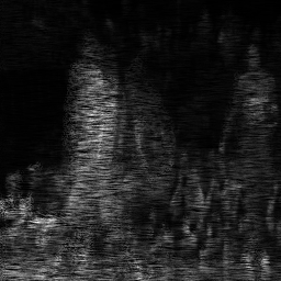
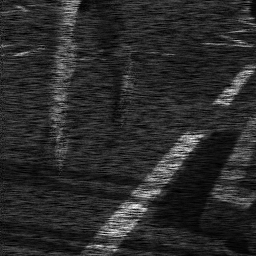
Measurement

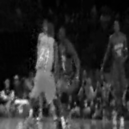
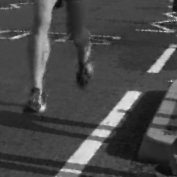
Reconstruction
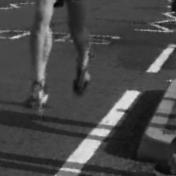
Ground Truth

Measurement
Reconstruction
Ground Truth
Measurement (perturbed)
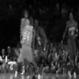
Reconstruction


Mean PSNR Across All Scenes
Per-scene PSNR breakdown (4 scenes)
| Scene | I (PSNR) | I (SSIM) | II (PSNR) | II (SSIM) | III (PSNR) | III (SSIM) |
|---|---|---|---|---|---|---|
| scene_00 | 28.83583466097646 | 0.8942128869007379 | 19.628746907852033 | 0.6299246978860197 | 28.661967596893607 | 0.888431847653619 |
| scene_01 | 20.88216606453536 | 0.7034055396617757 | 16.777755027773797 | 0.4868548118169957 | 20.84428515238867 | 0.7000468328132369 |
| scene_02 | 30.691990156584193 | 0.9154534922988713 | 24.827200485908673 | 0.8474444214238722 | 30.012986873119104 | 0.908457497268565 |
| scene_03 | 35.81071472884463 | 0.9741879755737781 | 30.14980891279552 | 0.9504253169730846 | 35.67595393556099 | 0.9734564527392388 |
| Mean | 29.05517640273516 | 0.8718149736087908 | 22.845877833582506 | 0.7286623120249931 | 28.798798389490592 | 0.8675981576186649 |
Experimental Setup
Key References
- Llull et al., 'Coded aperture compressive temporal imaging', Optics Express 19, 10526 (2011)
- Yuan et al., 'Generalized alternating projection based total variation minimization (GAP-TV)', IEEE ICIP 2016
- Wang et al., 'Spatial-Temporal Transformer for Video Snapshot Compressive Imaging (STFormer)', ECCV 2022
Canonical Datasets
- Kobe, Runner, Drop, Traffic (grayscale SCI benchmarks)
- DAVIS 2017 (adapted for SCI simulation)
Spec DAG — Forward Model Pipeline
M(m_t) → Σ_t → D(g, η₄)
Mismatch Parameters
| Symbol | Parameter | Description | Nominal | Perturbed |
|---|---|---|---|---|
| Δx | mask_dx | Mask lateral shift (pixels) | 0 | 0.5 |
| Δy | mask_dy | Mask vertical shift (pixels) | 0 | 0.3 |
| θ | mask_theta | Mask rotation (rad) | 0 | 0.1 |
| Δt | clock_offset | Clock synchronization offset | 0 | 0.05 |
| d | duty_cycle | Shutter duty cycle | 1.0 | 0.95 |
| g | gain | Detector gain multiplier | 1.0 | 1.02 |
Credits System
Spec Primitives Reference (11 primitives)
Free-space or medium propagation kernel (Fresnel, Rayleigh-Sommerfeld).
Spatial or spatio-temporal amplitude modulation (coded aperture, SLM pattern).
Geometric projection operator (Radon transform, fan-beam, cone-beam).
Sampling in the Fourier / k-space domain (MRI, ptychography).
Shift-invariant convolution with a point-spread function (PSF).
Summation along a physical dimension (spectral, temporal, angular).
Sensor readout with gain g and noise model η (Gaussian, Poisson, mixed).
Patterned illumination (block, Hadamard, random) applied to the scene.
Spectral dispersion element (prism, grating) with shift α and aperture a.
Sample or gantry rotation (CT, electron tomography).
Spectral filter or monochromator selecting a wavelength band.